Training a GAN on Google Street View
My fall 2019 independent study focused on machine learning + art, and ended up training a Generative Adversarial Network on Google Street View images. Although the project was pretty time consuming, I got a lot out of it, and actually learned more about machine learning than I had anticipated, given the focus on applications. I ended up displaying some of my work at Bellevue Art Museum's 20under20 exhibition. The Jupyter notebook with the model can be found here.

What's a GAN?
A Generative Adversarial Network (GAN) is not a single machine learning network, as it name implies-- instead, it consists of two networks competing against one another. One of the networks is a generator that translates information into images, starting with random noise as input. The other network is a discriminator, which attempts to distinguish the generated images from the original training images. The competition between the two leads to the continual improvement of both models; loss from the discriminator is used to train the generator as well. The discriminator has an easy job at first, because random pixel outputs are pretty different from structured image-- however, it also has no experience with what a real image would look like. Over time, the discriminator improves with feedback from the training set (whether or not it was correct), allowing it to distinguish the fakes better and better. The discriminator also gives feedback to the generator, providing information on what a real image should look like.
If both sides continue to improve, the generated images should become increasingly realistic and indistinguishable from the training set.

This project would be my introduction to machine learning. Although it was heavily skewed to the applied side, I tried to learn as much as I could about GANs & high level concepts as possible. I focused on understanding the core ideas to the Keras Sequential API, which I would be using to build the GAN. I found the DCGAN tutorial on Google Colab to be very helpful, as well as several other introductory Tensorflow tutorials with the MNIST dataset and 32x32 CIFAR10 images.
It was while completing one of these tutorials that I came across the idea of using Google Cloud TPUs (specialized processing units) to train the model completely online. This way, I wouldn’t have to find computing hardware on my own, which was a relief. One of the biggest challenges up until this point had been finding the hardware necessary to work with images, which tend to be quite graphically intensive. One epoch of training for one of the tutorials, which should have taken about 10 minutes, took the whole night to run on my own.
The classic example of GANs training on handwritten digits- from the MNIST dataset.
I completed the Tensorflow on TPUs tutorial, and assembled my own GAN model in a Colab notebook. The model architecture was based mainly on Matthew Mann’s 256x256 generator. I identified 256x256 images as the smallest possible size that would still be effective at conveying a visual. All that remained was finding the right dataset to train on.
Intermission
Earlier on in the year I had been playing around with using Google Street Views to form collages (not related to my ML project). Inspired by videos such as Paraic Mcgloughlin’s Chase and the like, I was thinking about automating a collection process to get thousands of different frames centered on a vanishing point.
This process would use street-level imagery from the Mapillary API, and a ML horizon detection algorithm. The user would choose a set of places, my program would pull street-view images from those locations, align the perspective points, and then overlay them in a fast-paced sequence.
As I had carried out initial tests, however, it became clear that navigating to a fixed perspective was too difficult given the wide variety of Street View images; for my project to work, it would require a more homogeneous image set and abandoning the automated horizon detection part, relying on manual alignment.
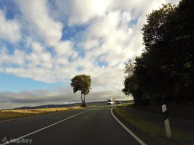
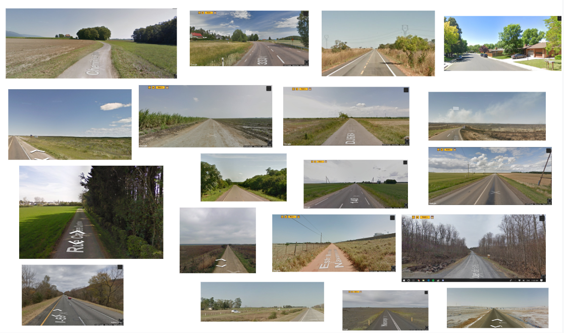
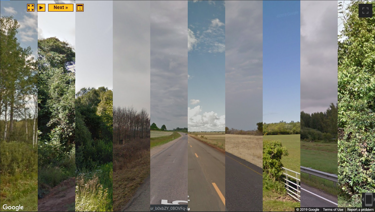
I did create several nice collages from this process, however:

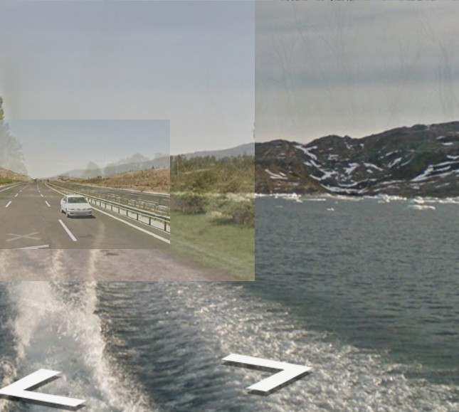
Certain biomes and landforms, tundras and deserts, or else forests with singular distinct masses, definitely mesh together better here. When I assembled the training dataset later, I would rely heavily on these aesthetic tastes in choosing images that I liked.
At this point I realized that Google Street Views collected in this way fit nicely as a standardized format into an GAN training set. If I could create a set of street view images that all shared a single perspective, that would help reduce the traditional issues associated with GAN training: different angles, subject matters, scale, and lighting.
With this set of images, I would be able to generate new landscapes, with the same perspective, but differing features. I could even maybe explore the application of them in a series, like the evolution of a landscape across time.
Data Collection
Yet I had no horizon detection algorithm in place, and using the Mapillary API to gather random, quality images was difficult. There were ways to specify latitude and longitude, but no easy way to change the angle at which the camera pointed. In addition, many images were a poor fit, due to issues with resolution, crowded city scenes, or a lack of a clearly defined horizon. I made the decision to brute force data collection so I could focus on the GAN itself.
I manually gathered the images from https://randomstreetview.com/, which displayed random Google Street View images from around the world. I physically identified the common horizon point with pieces of tape on my computer, and then took screenshots.
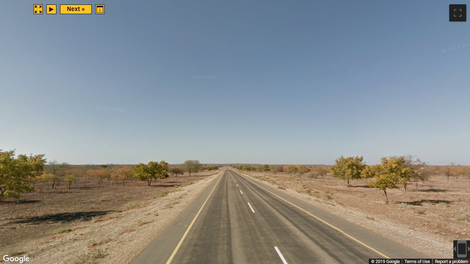
Over the course of about a week, I gathered an initial training set of about 150 images. I’d estimate that about 1 out of every 20 images had the appropriate lighting and environment to be screenshot-worthy. Although most GANs require at least 500+ images to produce realistic results, at this point I wanted to test out my model just to see if it would work.
Pillow
To process the data, I turned to Pillow, Python’s image manipulation library. Pillow would help me square the images, and resize them to the 256x256 size that I needed.
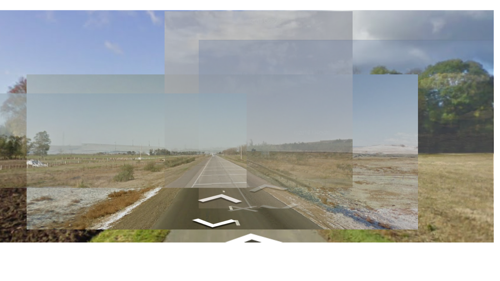
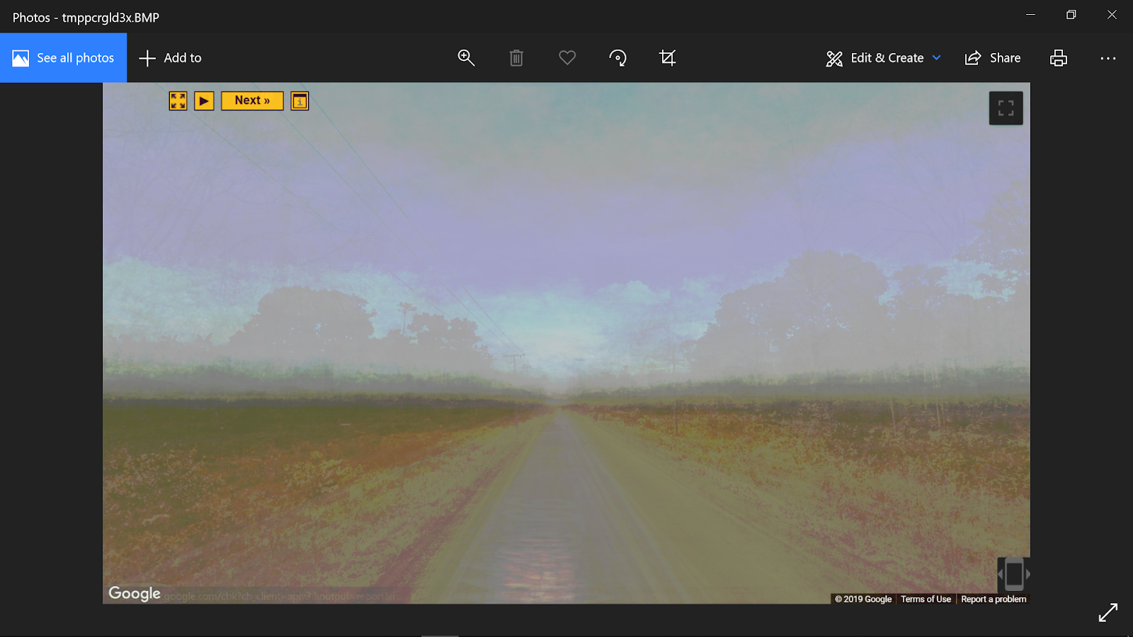
First, though, I found Pillow was really fun to work with. I lowered the alpha of the images and overlaid them on a single canvas object to create a translucent, painterly image:
This idea actually has a lot of potential and I keep meaning to come back to explore it.
I became quite interested in the applications of Pillow alone at this point, and I generated several different collages from the set just for fun before I got to the ML part of the project. That made a nice first post for the blog.
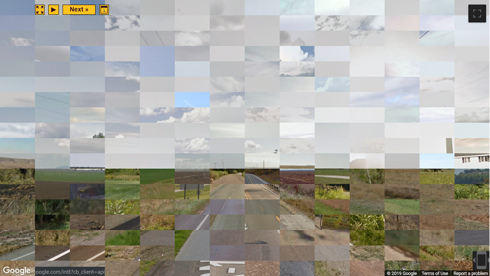
Each collage had a certain number of horizontal divisions and vertical divisions, and pulled tiles from random images:
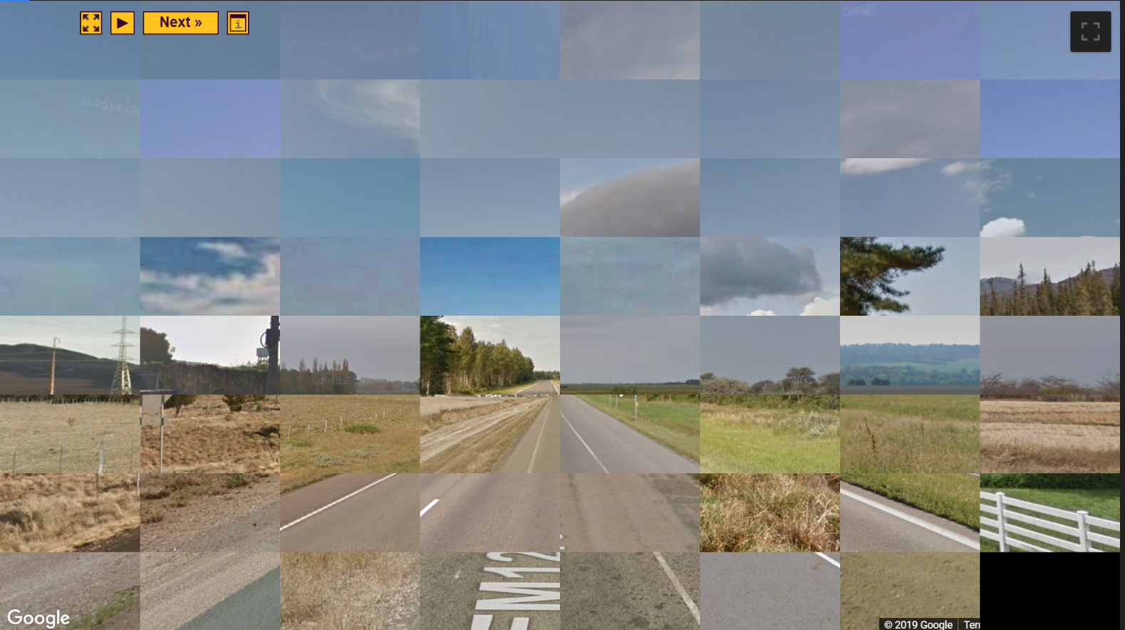
Off by one errors for the right bottom corner.
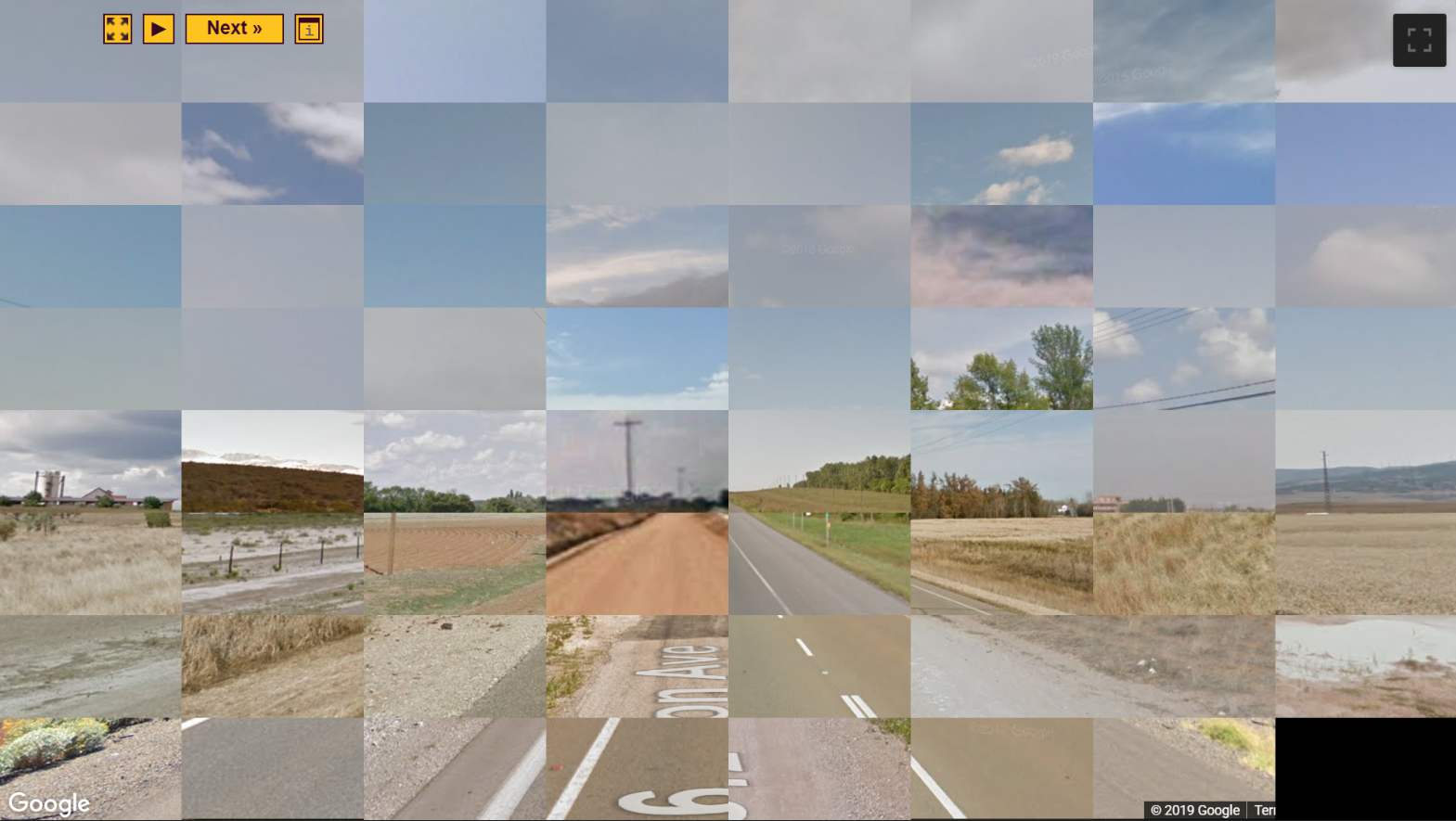
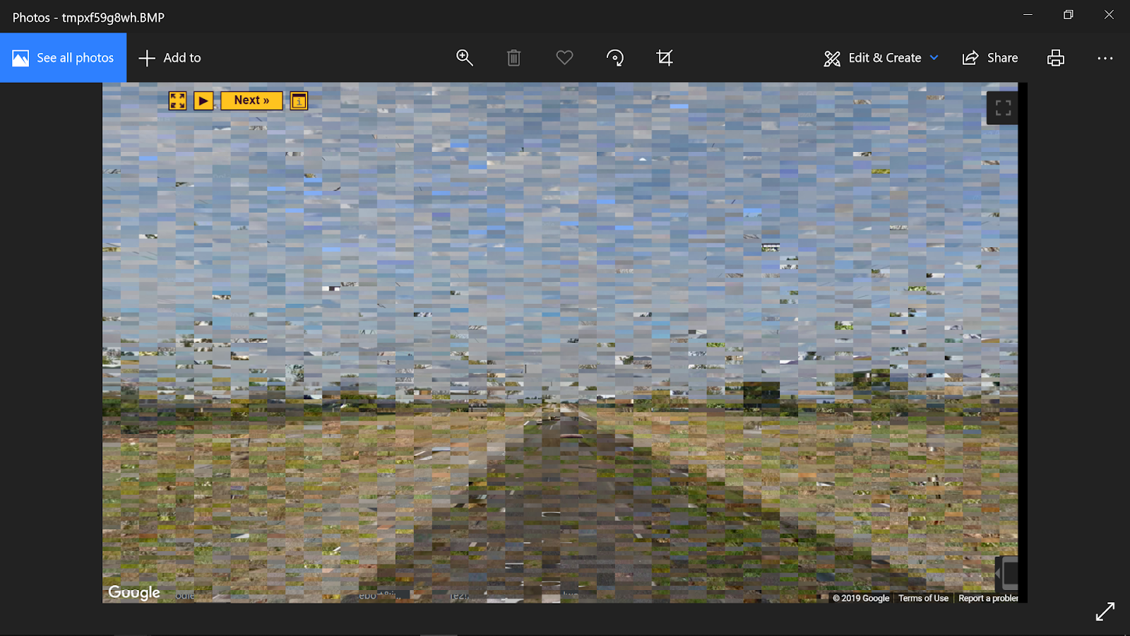
I looked for a brightness level of each image square within a certain range to achieve visual uniformity. This really just added a flat, washed out feel for the collages, however; I wanted a more dynamic range of brightnesses and more representative colors. I tweaked my collage generator to instead map the brightness level of a specific squares to the brightnesses of a representative image from the set, so that the resulting collage would appear closer in style to real life. This resulted in much better results:
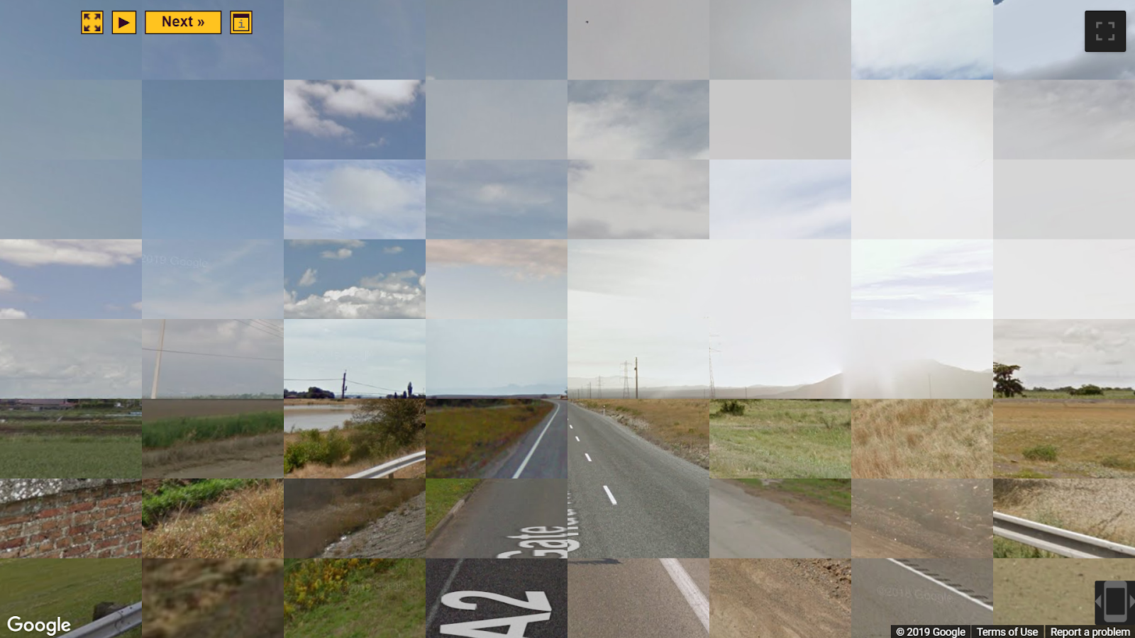
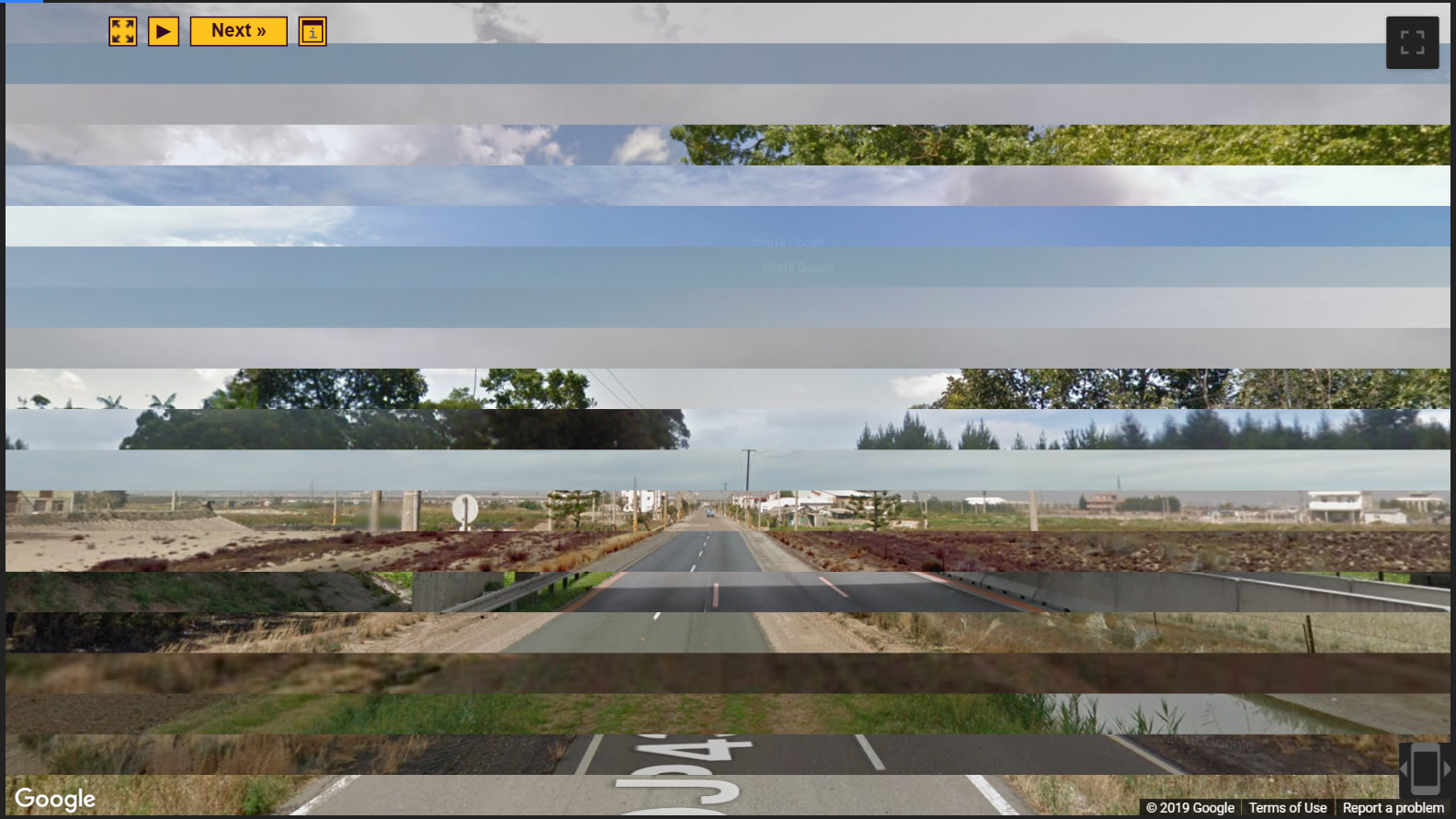
I really like these collages and the level of detail achievable with them; they also carry the same sense of wonder that I wanted to achieve with my ML work later. There was a lot of room for variation with the tiling and I played around with it:
GAN256
And back to the machine learning.
Using Pillow, I formatted the 1920x1080 screenshots into 1024x1024 square images, and then downsized to 256x256 so that the model could run on them. I uploaded the images to the Google Drive, configured a few things, and began to train the model on Google Colab.
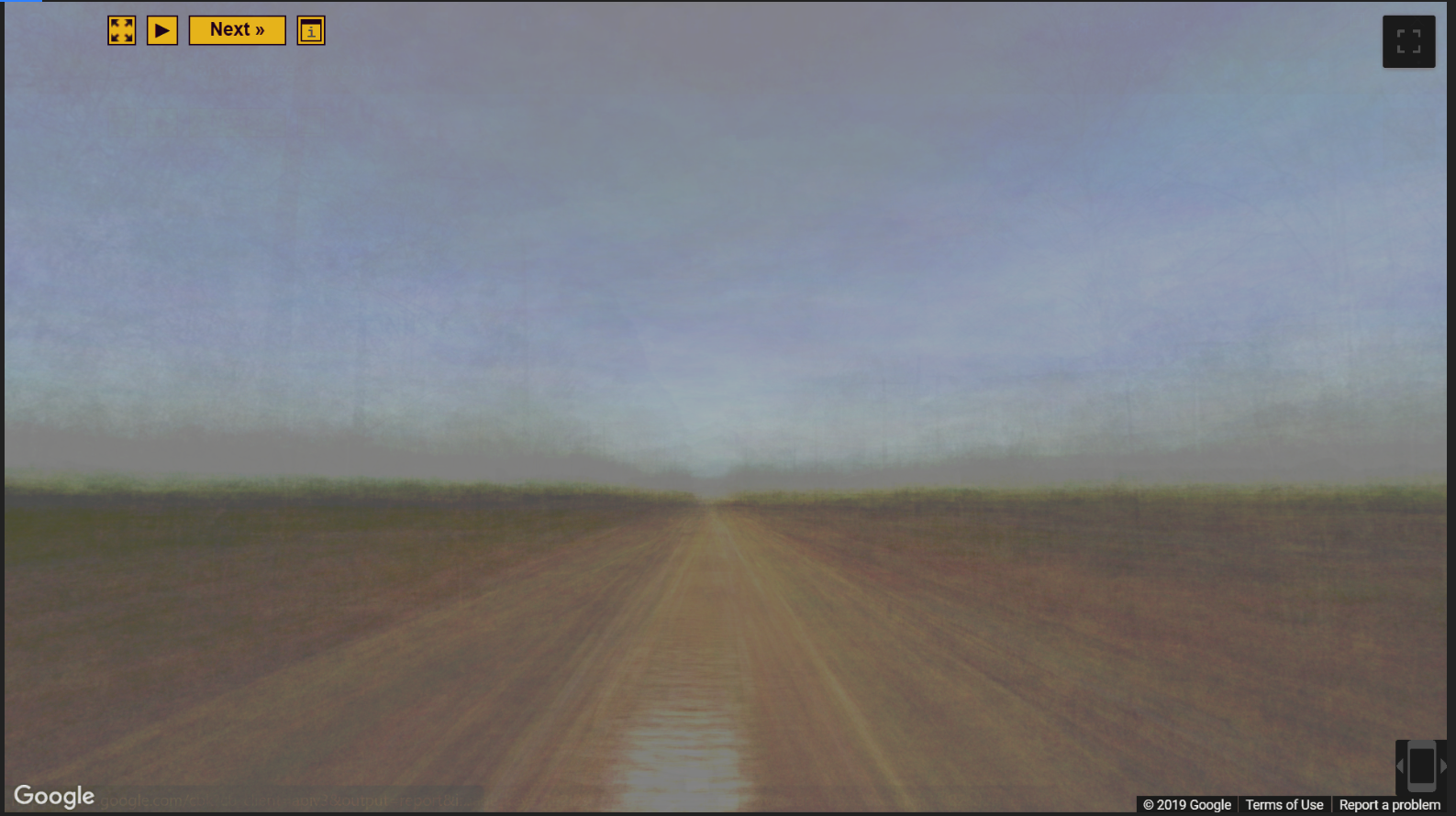
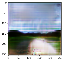
Here are the first and last images from the 1st training run I saved:

Exciting! Way too dark, and lacking structure, but there’s something appealing about it, even if its not intentional. You can’t really expect detailed results from the first few training steps.
These early images reminded me of Impressionist work.
Joseph Turner’s landscapes:
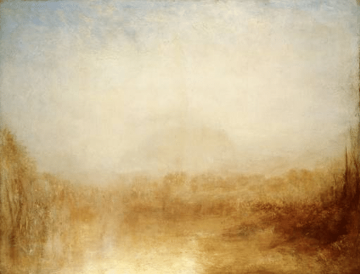
GAN generation in general seemed quite Impressionist-- and not only because of its blurriness and the forgiving nature of such art. The errors made are exciting and familiar as the generator strives to learn the image.
The network isn't working from an analytical perspective-- here's a oblong green circle 23 by 75 pixels wide-- but instead maximizing the convincing qualities of it to beat the discriminator. It captures the essence of a particular angle on a particular day in the way that Impressionism does, more than it captures trees as trees and bushes as bushes.
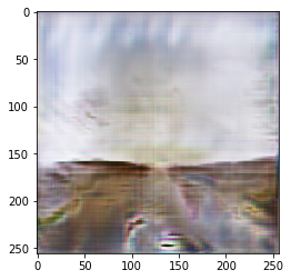
I did another training run, going a little further this time and letting the program run overnight:

I made a lot of silly mistakes throughout the process, but one of the more important ones was that I didn’t write a save function for the model until much later, which would have allowed me to train the model over several sessions and save the weights in between. This meant that my early runs were all very short and made little progress-- however, it was still exciting to see the initial development of any model. I later realized that the visual range of the images that were produced in these early runs meant that the model didn’t really train during any of these runs, but I think these were pretty interesting to look at; like underpainting or a watercolor wash.
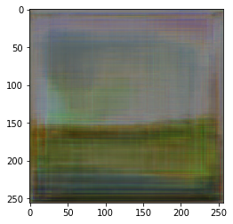
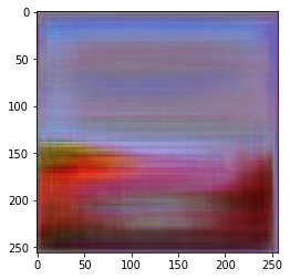
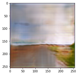
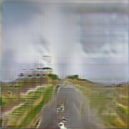
On my third training run, I let my computer run overnight, finally breaking some ground, and produced a much better training result:
Still extremely scratchy, you can start to see the ground/sky distinction forming. I was initially put off by how vivid the colors were at this stage but they would soon improve greatly in realism and coherence. You can see how the colors translate both vertically and horizontally and produce grids where the colors intersect. This is due to the way that the model interprets the image-- it might be because of the kernel size and striding.
This is where I began to make my modifications to the model. Having harsh labeling (1 = real, 0 = false) can apparently cause overcorrecting, making it detrimental for the learning of the generator. To combat this, I changed the hard 1 and 0 labels to soft labels (values ranging between 0-0.1 and 0.9-1), and incorporated noise.
Another modification I made was the size of the kernels, which are (almost) small arrays used to read the image matrices and then used to iteratively stacked to decipher image features. Using larger kernels increases the amount of information read, but slows down training. Originally, the model used 3x3 kernels, but I ended up using rectangular kernels because the landscape features were more horizontally oriented than vertically.
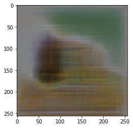
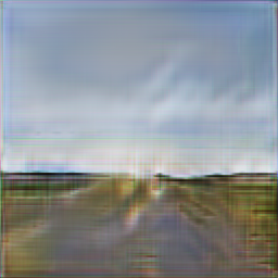
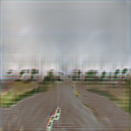
Here I change to 7x3 kernels:
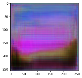
You can see the grid patterns have flattened horizontally. Things appear closer to the ground, and the horizon is better defined.
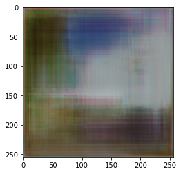
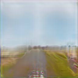
Before this next run, I have updated the images to include the full set of 350 screenshot (an image data function within the code also produces left-right mirrors of the original dataset, bringing the total to 700). I also change again to 7x4 kernels, which considerably slow each step but greatly improve the quality:

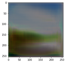
You can see that the edges look a lot smoother, and the colors are in more discrete clumps. The sky-ground distinction is also made, but there’s a lot of unnatural variation that I’d like to get rid of.
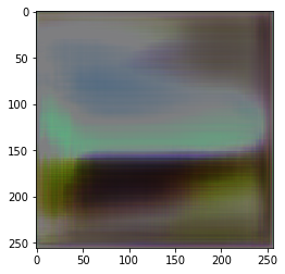
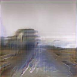
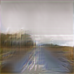
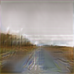
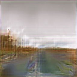
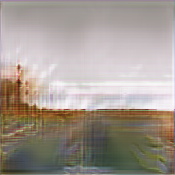
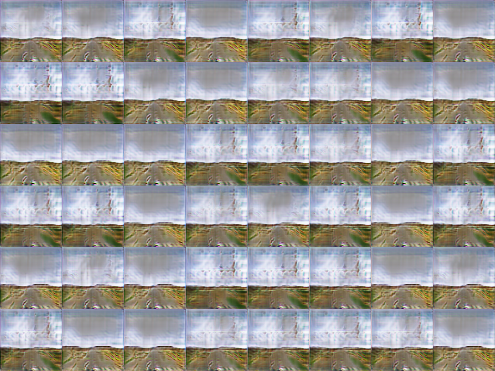
From this run on, I begin saving the model, allowing runs over longer periods of time than a single night. I also double the filter count for each layer, which decreases blurriness at the cost of increasing the number of parameters and run time:
I was very satisfied with the level of detail achieved by that last image, although some of the earlier images (the 4th) had very deep color contrasts that were quite beautiful.
I was very happy with the level of detail in the sky (look at the 3rd one!) but at the same time, small distortions began to appear in the model at this point. I kept running the model, hoping that they would eventually go away.
After a while admiring the different landscapes and colors that were forming, I decided to make a very important change; keeping the same random noise pattern as input into the model for every step in the model. This allows me to track a single “point” as the model continued to evolve, creating a chronological progression of the image. This would allow me to maintain some visual consistency from step to step, and track the emergence of different elements more closely.
Due to the interpretive process of the GAN, different familiar elements would often emerge; it would move from one recognizable shape into another, as the generator adapted against the discriminator and produced new patterns of imitation.
What seems like a large deciduous tree gradually morphs into a canyon like structure over a series of steps.
I decided to capture these in progress motions in gif format.
This would look similar to other generative projects that would explore a single latent space (essentially all of the different noise inputs possible) with a fully trained model. I was very excited about this possibility, because that would mean I could show the landscape as it morphed from one familiar scene to another. Yet when I tried this original idea with my model, drawing different images from a single version, there wasn’t enough variation for any single version of the model to make it worthwhile.
At any single stage, the generator’s concept of the landscape was quite specific, and it was the discriminator’s feedback that caused this concept to evolve over time.
So instead of moving around the latent space of a single moment of the model, I tracked a single point in latent space as the model itself changed over time. This actually produced really nice results immediately, to my own surprise. (Note that this was actually quite early in the model generation, so it is still somewhat blurry).
I would gradually improve on this process and make several more continuous gifs.
This one loops back and forth:
And finally, I produced a random “flash” gif, giving the illusion of forward motion:
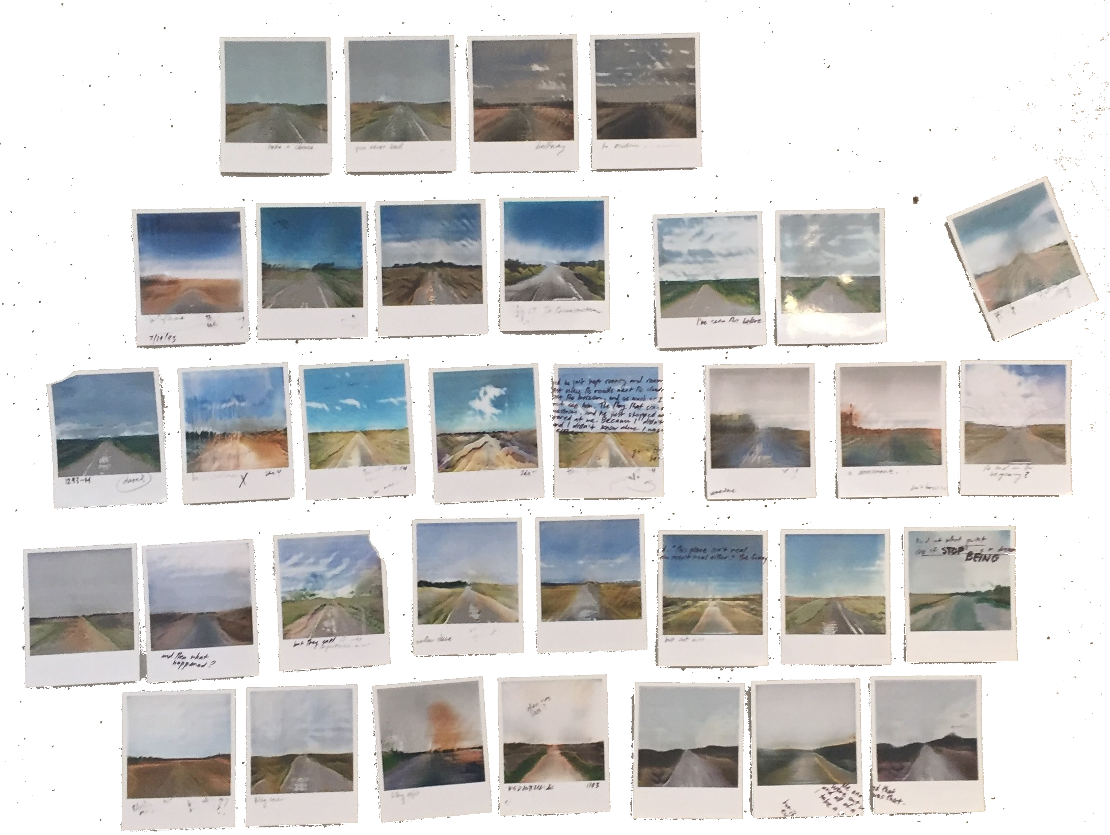
I ended up presenting the following final pieces for Midwinter Arts Show and some local exhibitions (click to view up close.):