Terraforming Mars with Pix2Pix and Satellite-Elevation Image Pairs
Eric Xia, Taj Gillin, Julian Dai
Dependencies
All necessary dependencies can be installed in a conda environment via the environment.yaml file included in the repository. These include the packages pytorch::pytorch, torchvision, scikit-image, numpy, matplotlib.
Introduction
Our project implements the GAN architecture described in the Pix2pix paper for the task of “greening” extraterrestrial imagery to earth-like satellite imagery, accomplishing this through the usage of elevation data as label maps. This is a supervised task involving synthesis from pre-existing label maps.
We arrived at this specific goal after settling on Pix2Pix as our architecture. While we initially considered doing image colorization, we found this task to fall in the sweet spot between originality and tractability. There exist large amounts of accessible elevation and satellite data (particularly on Mars), and the idea of using this data to terraform other planets was exciting.

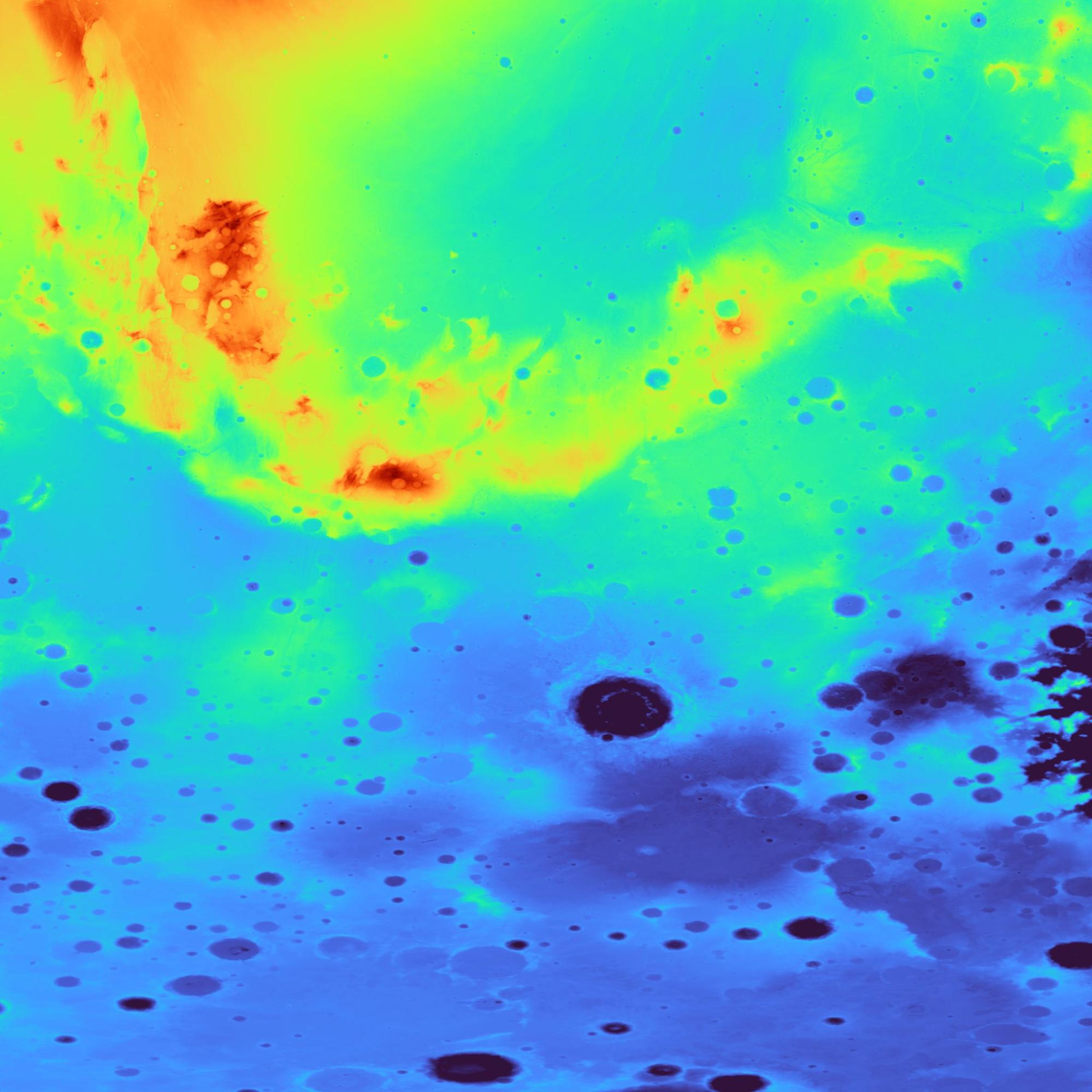
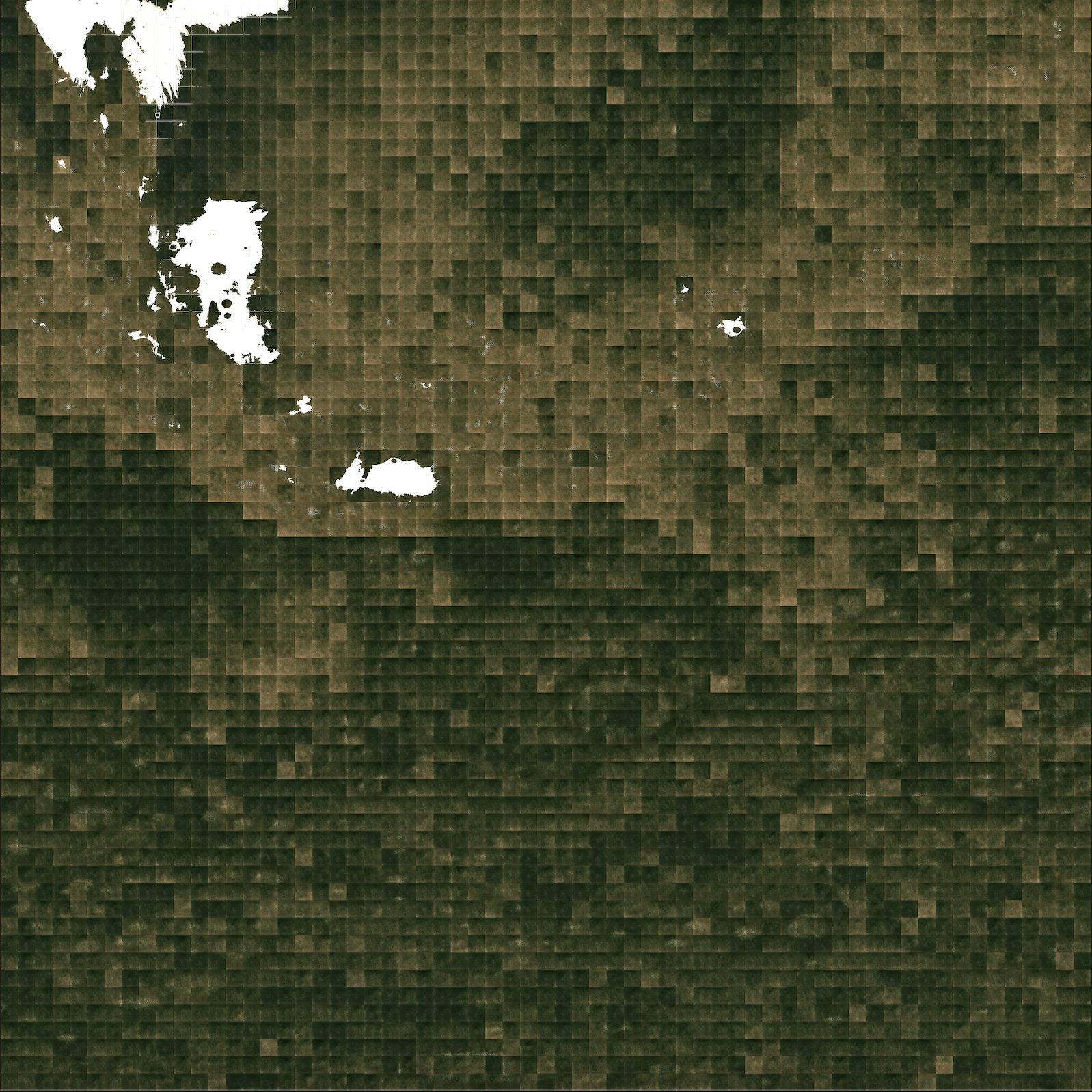
Final result: Elevation map and generated satellite imagery. South of Tharsis Rise & Argyre Basin, Mars
Methodology
Data Collection:
The elevation data comes from the Shuttle Radar Topography Mission, accessed through Google Earth Engine at 200 meter per pixel scale. Our elevation data from Mars was the same resolution and sourced from the Mars Orbiter Laser Altimeter, collected between 1999 and 2001. Thus, we ended up with 51.2km by 51.2km squares for 256x256 images. We collected these in 614.4 km by 614.4 km (12 x 12) and 768 km by 768 km (15 x 15) squares.
Although we planned on using LANDSAT satellite imagery from Earth Engine as well, creating cloudless image mosaics for large areas was time-consuming and difficult.. We ended up using images from the 2020 Sentinel-2 Cloudless Mosaic, licensed under CC BY-NC-SA 4.0.
Our final dataset consisted of satellite and elevation data retrieved from mountainous temperate regions around the world, and covering about 5.7% of global surface area. These were retrieved in 12 x 12 or 15 x 15 squares from the following regions:
To ensure 51.2km by 51.2km squares, we adjusted the longitude of regions by interest by the Haversine formula. QGIS was used to uniformly colorize elevation maps from a 0 to 9000 km scale. gdal_translate was used to resize the images, and Python Image Library for conversion to JPG.
Preprocessing:
We compiled the data into elevation maps and satellite image pairs labeled by place of origin. We then converted all image data from numpy arrays to PyTorch tensors. Following the pix2pix paper and Tensorflow implementation, we also applied random jittering and mirroring to preprocess the training set. The random jittering and mirroring can be described by the following algorithm:
Finally, we created a wrapper GetDataset() function that would allow us to compile data from specific regions according to the file path.
Architecture:
We initially implemented a naive Conv2D and Conv2DTranspose network in Tensorflow to test the ability of our model to learn satellite imagery from elevation maps. Conditioned on elevation maps, this network used MSE loss between the generated and real satellite images.
The architecture is shown below, and consists of 4 downsampling and 4 upsampling layers.
After 4 epochs training on the California dataset (144 elevation-satellite image pairs, 576 steps), we were able to learn the following results after 4 epochs:
This was enough to validate our concept as potentially successful. In order to achieve higher detail, we moved to the conditional generator-discriminator architecture we had originally planned on using.
For our main architecture, we followed the pix2pix paper (https://arxiv.org/abs/1611.07004), referencing the structure of the Tensorflow implementation but working in PyTorch. Our rationale for doing this was the vast amount of existing Tensorflow implementations, and the fact that the original PyTorch code was not structured for a specific implementation. Near the end of the project, we faced difficulties with implementing the generator and discriminator and referenced the original PyTorch implementation (expanded on below). We created a conditional generative adversarial network, with a U-Net for the generator and a convolutional PatchGAN discriminator.
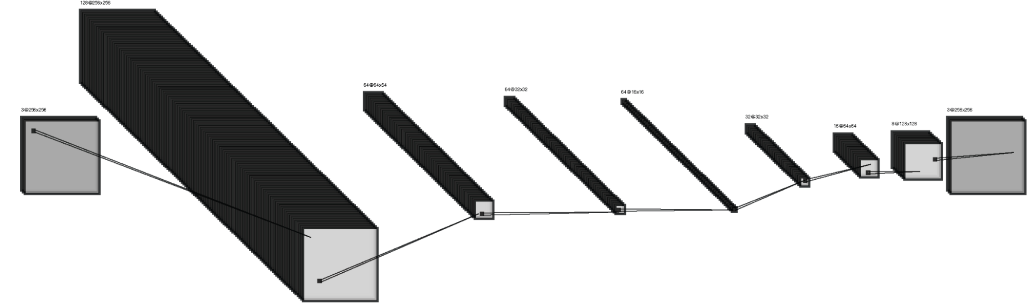
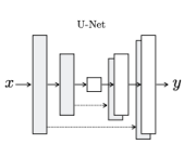
→ Generator (U-Net): The U-Net architecture was first introduced for biomedical image segmentation, but has quickly been adopted for a variety of image generation tasks. It is an encoder-decoder architecture with skip connections between mirrored convolutional layers in the encoder and decoder stack. The PyTorch model as implemented has 8 down layers and 8 up layers, as does the Tensorflow one.
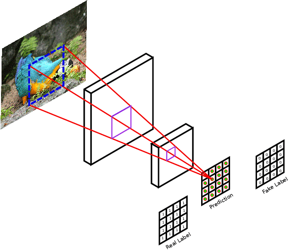
Discriminator: The PatchGAN discriminator classifies whether 70x70 image patches are real or fake using a convolutional architecture. Unlike a traditional discriminator, which has a single output, the output here is a 30x30 matrix, where each cell represents the classification of a patch. For real images, the ideal output should be full of 1s; for the generated images, it should be 0. Our PatchGAN implementation used 3 layers, each decreasing in resolution while increasing the number of filters.
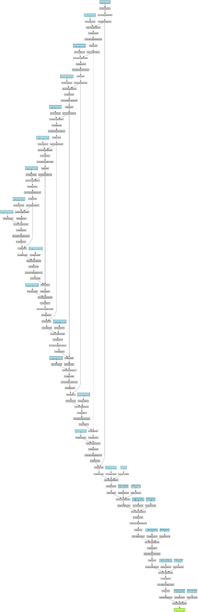
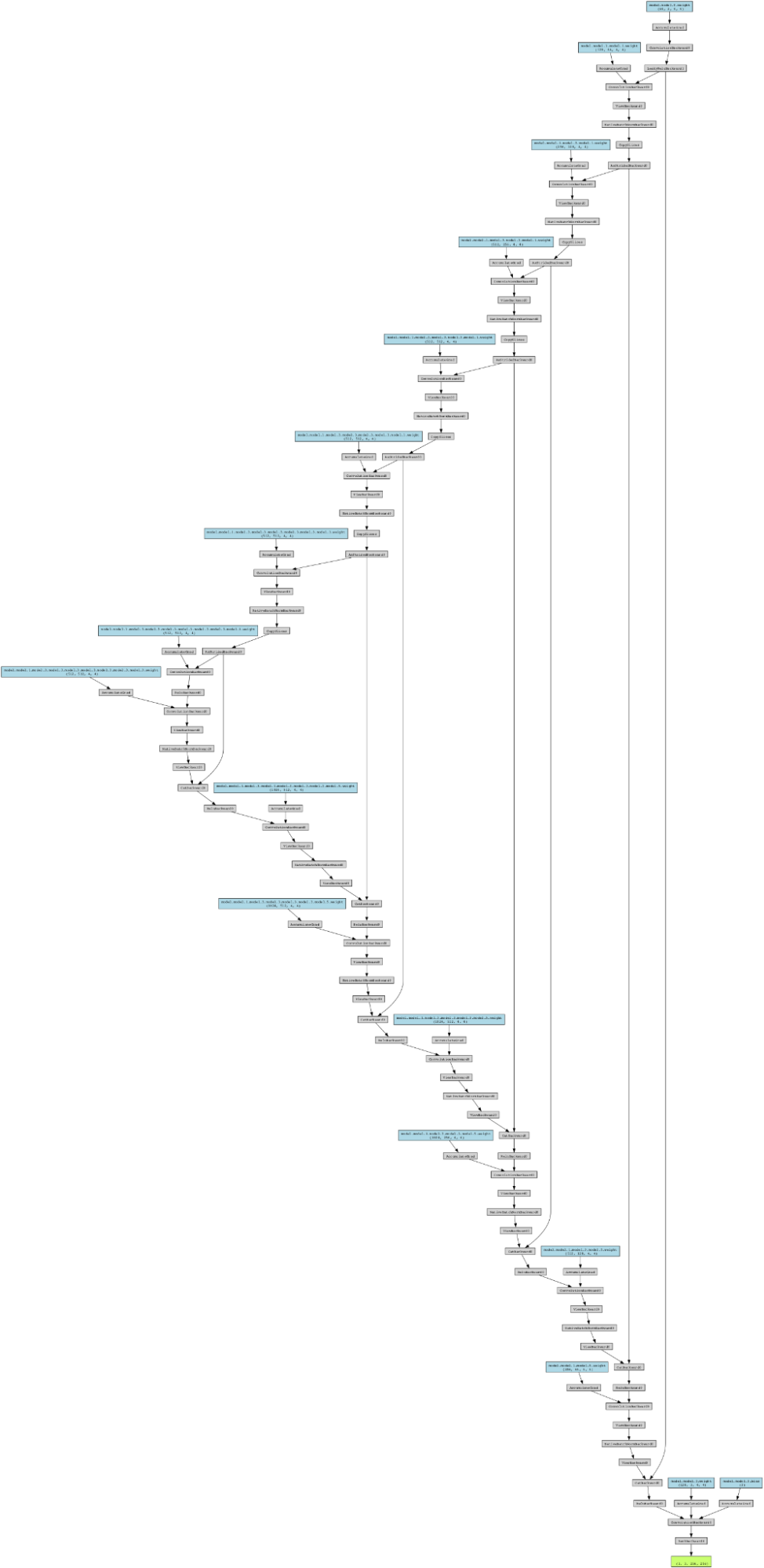
Torchviz visualization of graph execution: Discriminator and Generator. We can see the encoder-decoder architecture in the U-Net, and the downsampling in the PatchGAN.
Loss Function
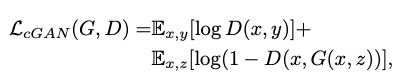
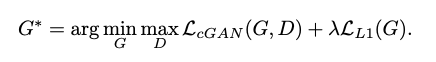
We used the standard overall cGAN loss:
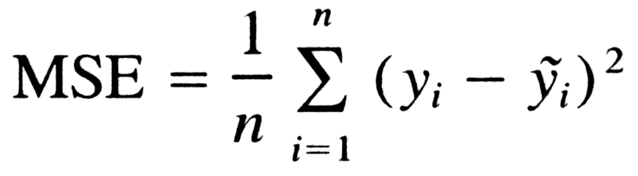
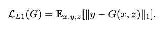
Where G minimizes the function against an adversarial D that tries to maximize it. Following previous approaches, we also add L1 loss to our final objective function as previous approaches have found it beneficial to add some form of traditional loss. L1, or Absolute Error Loss, is defined as follows:
Our final objective function is thus
where lambda is a hyperparameter.
Challenges
The biggest challenge we faced was the adaptation from Tensorflow to PyTorch. We were able to run the Tensorflow code on our dataset and get reasonable results quickly. However, we saw that Tensorflow abstracted a lot of the work out of creating architecture.
We faced issues with backpropagation and calling the gradient step correctly. In Tensorflow, the process of applying gradients is straightforward, with two separate GradientTape objects for the generator and discriminator and calls to apply_gradient. However, in Pytorch, we used disc_loss.backward() and gen_loss.backward() respectively. This caused problems with traversing the execution graph more than once, until we realized that the discriminator call on the generator needed to be detached in order to preserve the backpropagation process. As a result, our code now forward propagates twice, calculating the gradient and updating the discriminator first, then the generator.
Near the end of the project, we faced difficulties with implementing the generator and discriminator and had to reference the modified Pix2Pix PyTorch implementation. We traced the issue to the generator architecture. Unlike in Tensorflow, there is no way to specify SAME padding with a stride of 2 in the Conv2D or Conv2DTranspose methods. This is due to the controversial way that it is implemented in Tensorflow, where the padding can be uneven, and dependent on the input size. This meant that our attempts to implement the model sequentially were incorrect: often, the discriminator loss would settle at a fixed value while the generator would fluctuate, producing homogeneous green images.
We ended up referencing the UNetSkipConnectionBlock and UNetGenerator classes from networks.py in the original, which utilized a recursive structure to build the UNet. We fixed the hyperparameters to provide 8 up-down layers, 3 input channels, and 64 filters in the last generator and first discriminator layer respectively.
Moreover, we faced a problem with the normalization layers. The paper reported best results with a batch size of 1. The modified Tensorflow implementation used BatchNormalization, which accepted batch sizes of 1. However, Pytorch’s BatchNorm2D did not accept batch sizes of 1 due to not being able to calculate standard deviation. Referencing the NLayerDiscriminator class, we found that the original implementation used InstanceNorm2D, which we adopted as well.
With these changes, we were able to successfully run the generator, the discriminator, retrieve losses, backpropagate, and train the model.
A final challenge we faced was the long run times needed to train a GAN well. Due to these long run times, we were unable to make quick adjustments or fix bugs without waiting for the model to train. Our solution to this problem was to separate our code into cells in a Jupyter notebook. This way, we could make sure individual components of our code were working before we committed to running the entire model. This switch helped us catch some bugs in our data preprocessing as well as create a more organized overall model.
Results
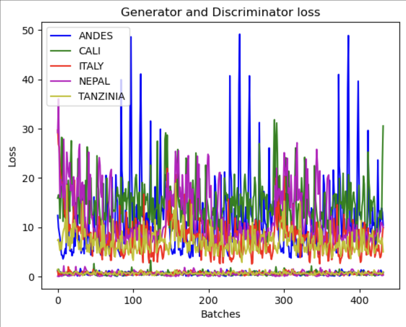
The plot above shows the generator loss (above) and the discriminator loss (below) across a few hundred batches for several different regions of data
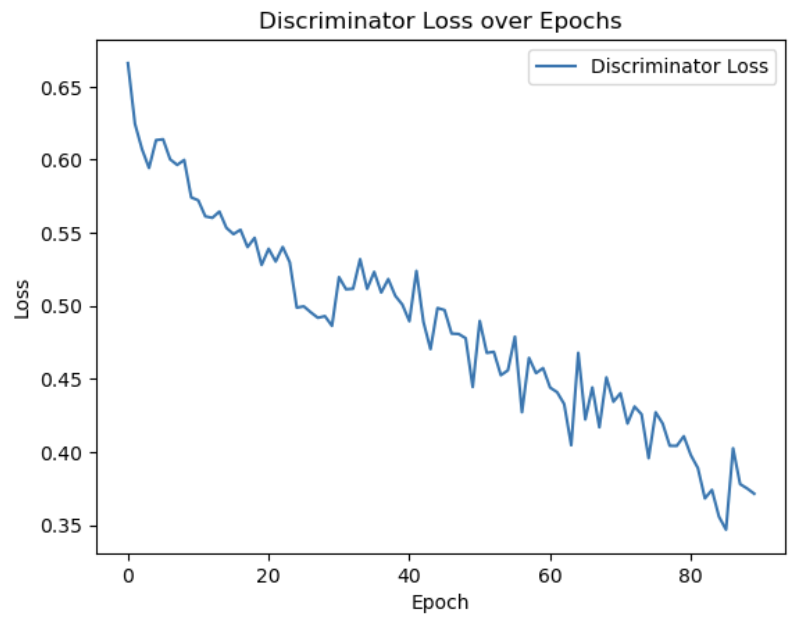
Above the generator loss is graphed over the epochs for a model trained 90 epochs (~100k steps).
Above the discriminator loss is graphed over the epochs for a model trained 90 epochs (~100k steps).
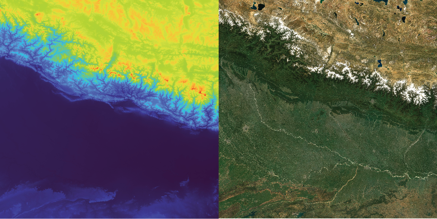
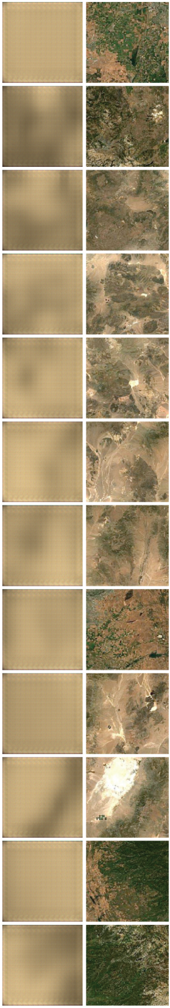
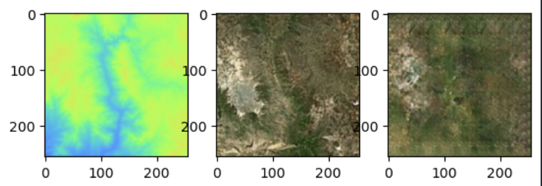
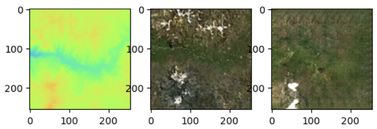
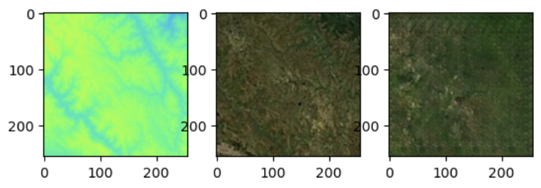
Above are elevation maps (left), their corresponding satellite images (middle), and the predictions generated by our model (right).
Reflection
Overall, we are very satisfied with the results of our project and feel that we achieved our target. By our evaluation of the generated terraformations, we believe that our model was able to learn mappings between elevation maps and satellite imagery that resulted in the generation of feasible results for what a satellite image of Mars would look like. We did not have a specific accuracy metric to test the performance of our models’ terraformation of Mars, as satellite images of terraformed Mars do not exist. If we had been unable to get elevation maps for Mars, our base goal was defined to be validation against Earth satellite images and we were able to achieve that above.
If we had more time, we would tweak the architecture of the model to experiment with how changing the model would affect the generated output. Furthermore, we believe that we could improve our model by adding latitude and longitude points as an additional conditional input to our generator to help the model learn the different correlations of elevation and satellite imagery at specific locations. Since this climate/ biome correlation can vary significantly depending on location, our model would be better suited to generate more accurate terra formations of Mars given a specific latitude and longitude. Furthermore, since the elevation on Mars have much steeper gradients than those on Earth, another step we could have taken in preprocessing to perhaps enhance the output of our model would be to normalize the elevation maps of Mars to a range that can be found on Earth, or alternatively, scale elevation maps of Earth to the steep gradients found in the elevation maps on Mars.
Ultimately, our biggest takeaway from the project was a familiarity with the entire lifecycle of a deep learning project. We learned a lot about project design, setting realistic expectations, researching other people’s work and adapting it, and working together in a team. In our experience, our work in CS has mostly centered on more algorithmic processes rather than experimental ones. As a result, we found it difficult at times to find a sense of direction when faced with issues in our project that we could not specifically identify. For example, we struggled for a long time when the discriminator loss for our model wasn’t changing. We were unable to locate potential sources of error, as we were not sure whether the error came from our architecture or backpropagation. We eventually found the issue to be an error in preprocessing, where certain image pairs were not being flipped together. Thus, another takeaway for us was learning how to troubleshoot and develop intuition about where to look when facing bugs or challenges.