Analogues of semantic and geographic space𓂁
I've been working on word golf for more than a year, so I definitely won't be able to go into detail about everything I've done. There are dozens of experiments with interesting results that have appeared! But at this point my current work seems like a good fit for blog posts, so I'll just start writing it up here, and gradually add older content if it feels interesting enough in comparison.
Disclaimer: there's a high level of intuition at play here. No number or scale can accurately represent the intricacies of a language, and a lot of this is highly speculative.
That being said, there's something about working with word models that appeals to me more than anything else. I term the process of filtering as sculpting: it's a negative process in the same way carving marble or whittling wood is. There's striving towards art involved, a perfect representation of the english language.I want to make beautiful models with coherent associations. I've made maybe three models to date. The current one being used in my model is GloVe after a long polishing process. The next one I'm working on is Word2Vec, which is a bit more recent.
There's a special excitement for me about word golf that I can't seem to be able to convey very well to others. When you click links you're literally jumping between points in wordspace. There's this whole analogy of semantic space to physical geography that isn't yet captured by anything that exists. I will set out to prove that this metaphor holds firm for models after applying dimensional reduction.
I'm using a commoncrawl word2vec model with a vocab size around 52k. Imports are gensim's KeyedVectors, the TSNE implementation from sklearn, and matplotlib.
            # coding=utf8>
            from gensim.models import KeyedVectors
            import numpy as np
            from sklearn.manifold import TSNE
            wv = KeyedVectors.load('w2v_base_2.kv')
            print(len(wv.key_to_index))
            X = wv[wv.key_to_index]
            tsne = TSNE(n_components=2)
            tsneX = tsne.fit_transform(X)
            np.savetxt('tsne.txt', tsneX, fmt='%f')
This gives us a list of coordinates for our words. We can then establish a compass of sorts by taking a look at the outermost points:
            sX, sY = set(X), set(Y)
            s_sX, s_sY = sorted(sX), sorted(sY)
            west_mosts = [X.index(s) for s in s_sX[0:10]]
            east_mosts = [X.index(s) for s in s_sX[-10:-1]]
            south_mosts = [Y.index(s) for s in s_sY[0:10]]
            north_mosts = [Y.index(s) for s in s_sY[-10:-1]]
So our compass looks like this:
            WEST: bluest,tourniquet,tourniquets,sweetens,sweeten,
            sweetened,sweetening,dormancy,dormant

            EAST: isn,doesn,weren,shouldn,couldn,hadn,wouldn,didn,hasn

            SOUTH: gobbled,gobble,gobbling,devours,devouring,devoured,ranch,ranching

            NORTH: smothered,suffocate,strangling,suffocated,strangled,
            asphyxiated,fending,fended,egged
My intuition: the W/E axis for the english language goes [object, hot, free <--> object, cold, determinate] and the S/N axis goes [active, life, relaxed <--> active death, formal]. Is this just speculation? Yes, but I looked at like five different samples and they were able to convince me of my own hypothesis. Haha. If it does hold, it is a really interesting result though, it seems to hint at a universal scale upon which all words are based. I should do a blind trial at some point, and also look at other reduced models to see if these pairs of axes have some universality to them.
I'm much more confident in the hypothesis that the north direction tends to have more formal words and the south direction less. Anyways, let me explain what I'm working on right now.
actually playing golf
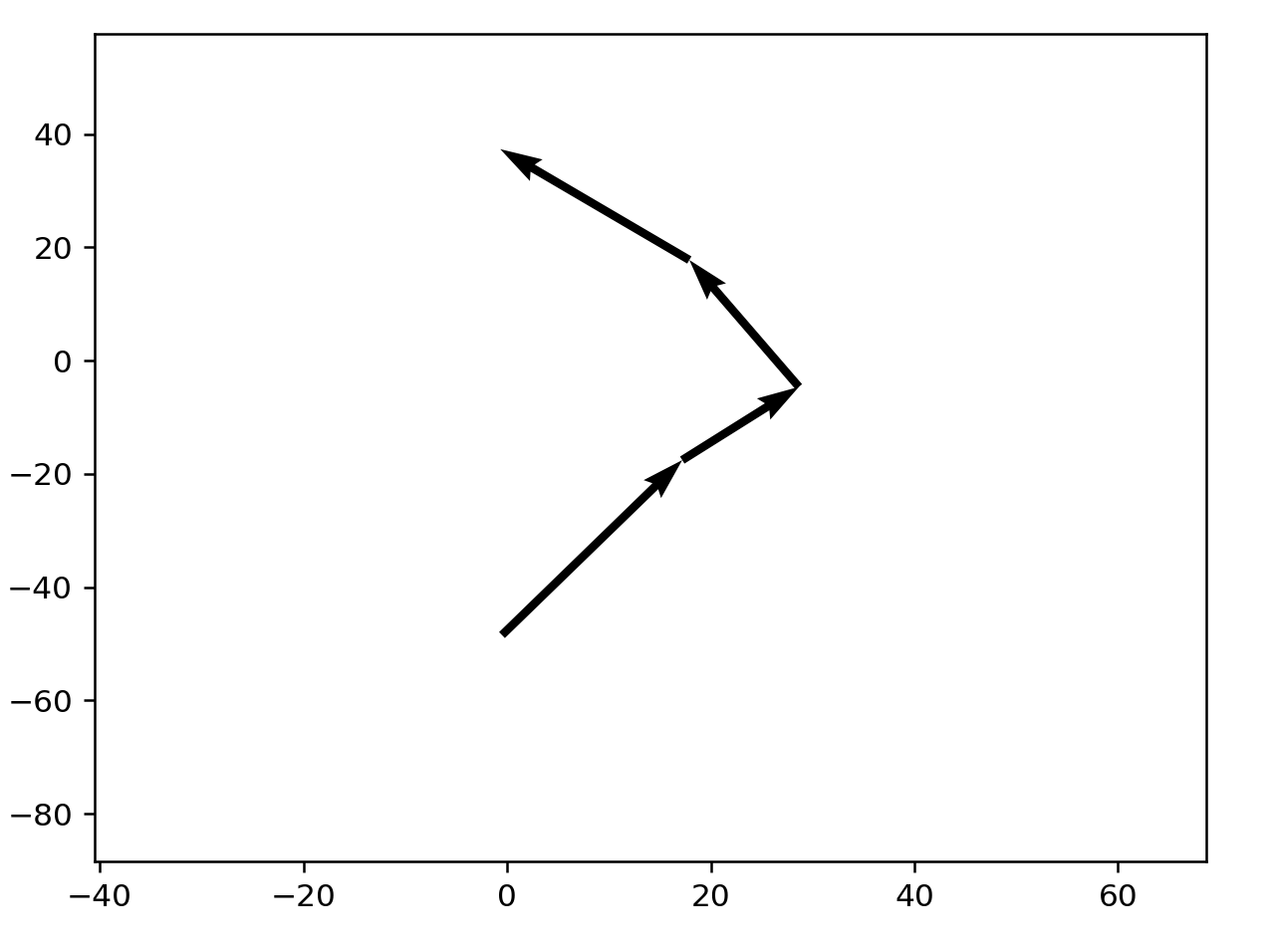
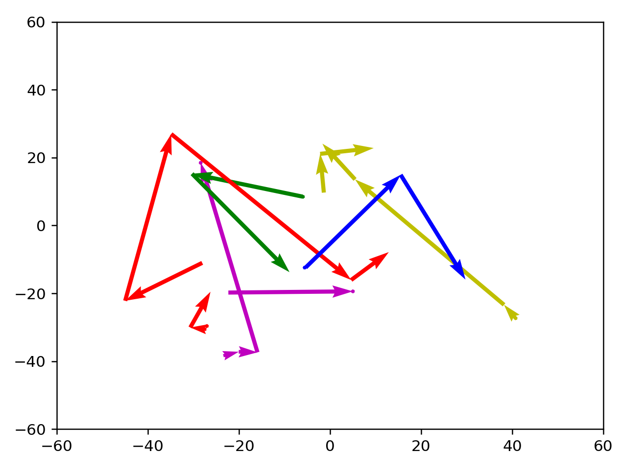
We can now visualize previous runs through the current word golf format (top 27 neighbors out of 100 presented in a grid, shifting through them until you get to the target), to see if this golf analogy holds up. First I'm just converting these points to Geogebra and pasting them in one by one. So here's one pretty standard run I completed converted and visualized:
r = ['department', 'board', 'body', 'black', 'silk', 'cotton', 'wood', 'copper']
for i, w in enumerate(r[:-1]):
    print(f"Vector(({tsneFlat[wv.key_to_index[w]][0]},{tsneFlat[wv.key_to_index[w]][1]}),({tsneFlat[wv.key_to_index[r[i+1]]][0]},{tsneFlat[wv.key_to_index[r[i+1]]][1]}))")

#Vector((-2.164832,17.089323),(0.278164,15.964342))
#Vector((0.278164,15.964342),(-12.965697,-6.741527))
#Vector((-12.965697,-6.741527),(-8.160164,-34.544804))
#Vector((-8.160164,-34.544804),(0.880635,-35.023899))
#Vector((0.880635,-35.023899),(-17.483561,-34.581875))
#Vector((-17.483561,-34.581875),(-14.143103,-27.133062))
#Vector((-14.143103,-27.133062),(-27.333059,-16.398949))
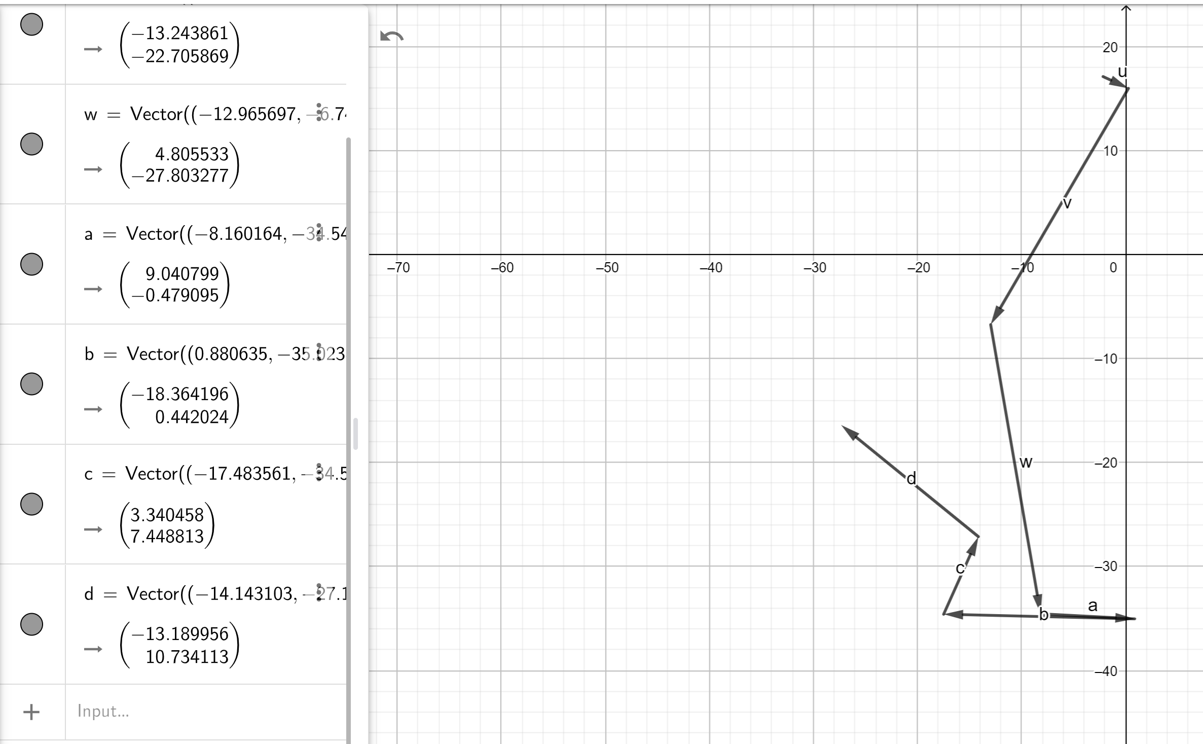
Okay, hey, this is actually a lot like normal golf, especially that first stroke towards the target! It seems like interesting enough to warrant writing a viz script for. Writing this kind of thing takes longer than I would like but quiver yields a result:
startx, starty, endx, endy = [], [], [], []
for i in range(0, len(xs)-2):
    print(f'Vector(({xs[i]}, {ys[i]}),({xs[i+1]}, {ys[i+1]}))')
    startx.append(xs[i])
    starty.append(ys[i])
    endx.append(xs[i+1])
    endy.append(ys[i+1])

for i in range(0, len(endx)):
    endx[i] = endx[i]-startx[i]
    endy[i] = endy[i]-starty[i]
import matplotlib.pyplot as plt

#startx and starty represent the points before
#print(startx[0], starty[0], endx[0], endy[0])
plt.quiver(startx, starty, endx, endy, angles='xy', scale_units='xy', scale=1)
plt.xlim(min(startx)-3,max(startx)+3)
plt.ylim(min(starty)-3, max(starty)+3)
plt.show()
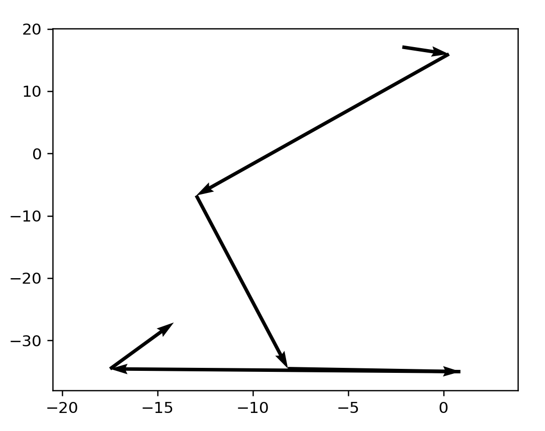
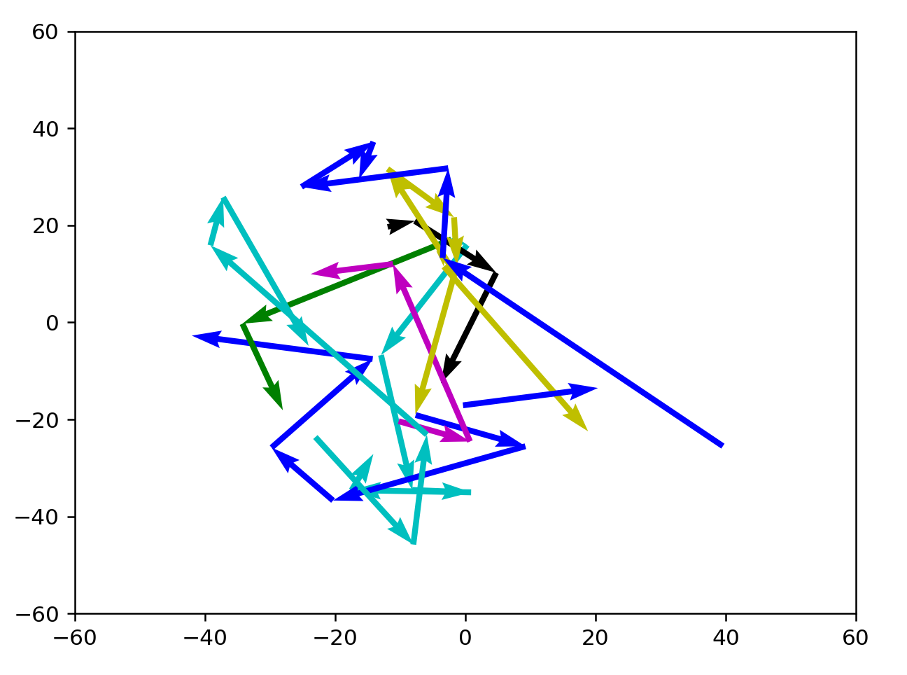
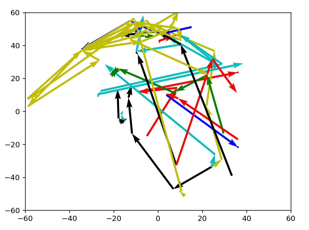
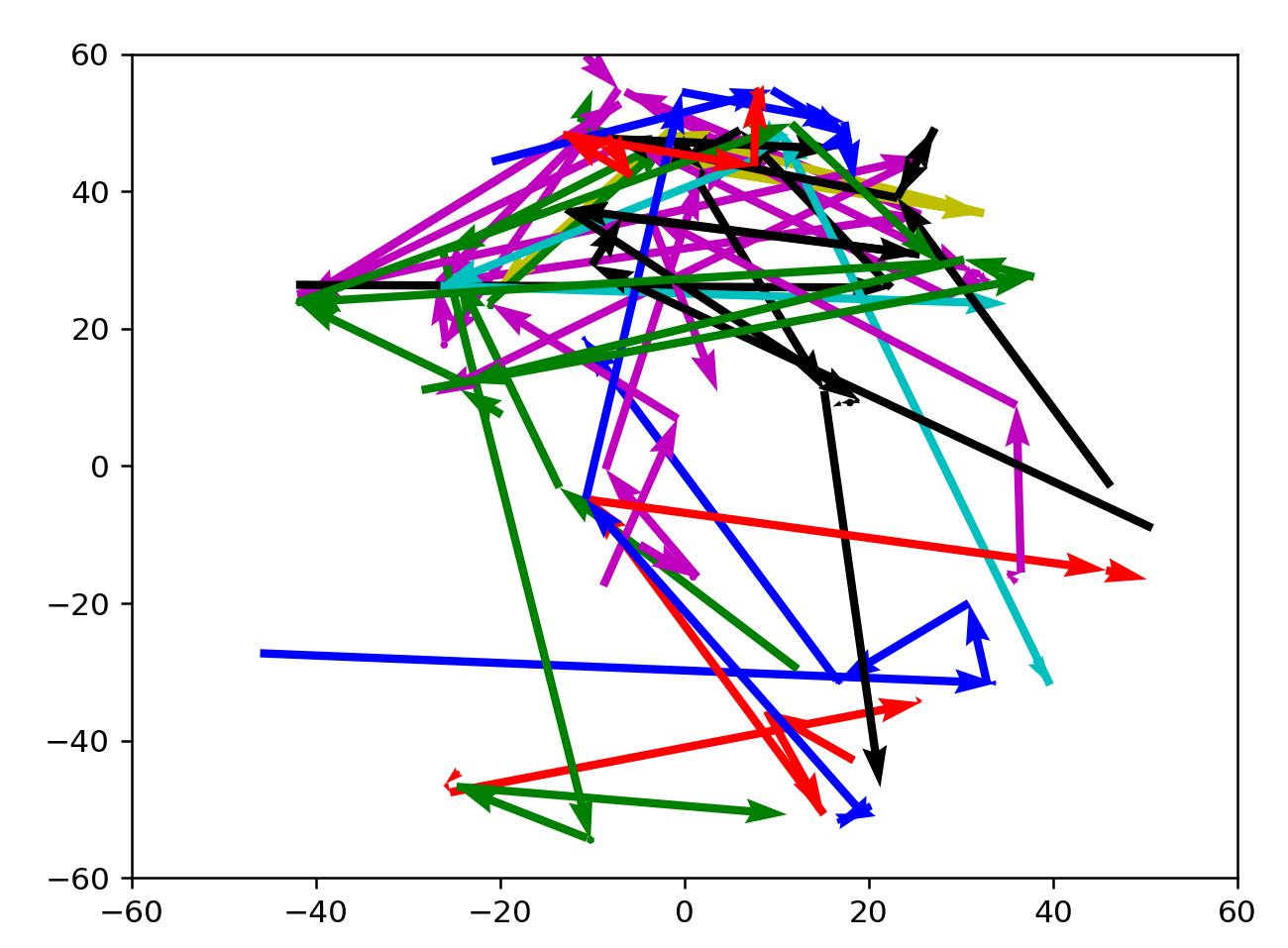
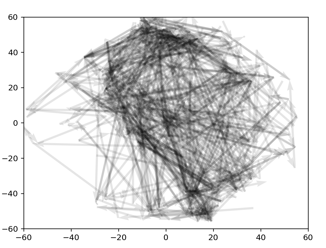
Now that we've established our script works let's try visualizing more.
Unfortunately there doesn't seem to be intuition here, with first arrows heading in opposite directions from the target word. Random samples from the completed runs:
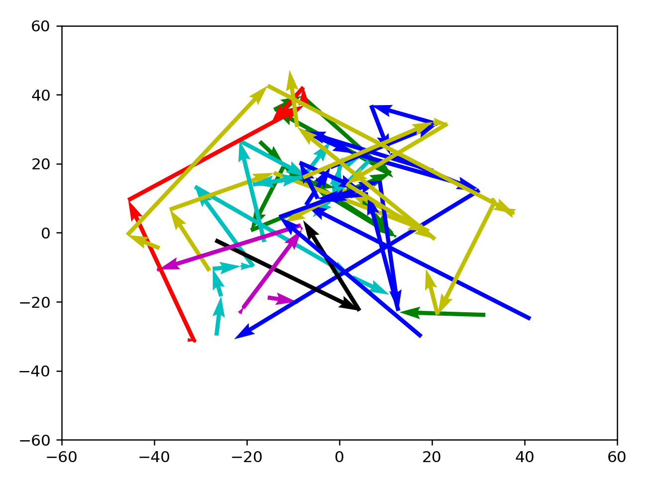
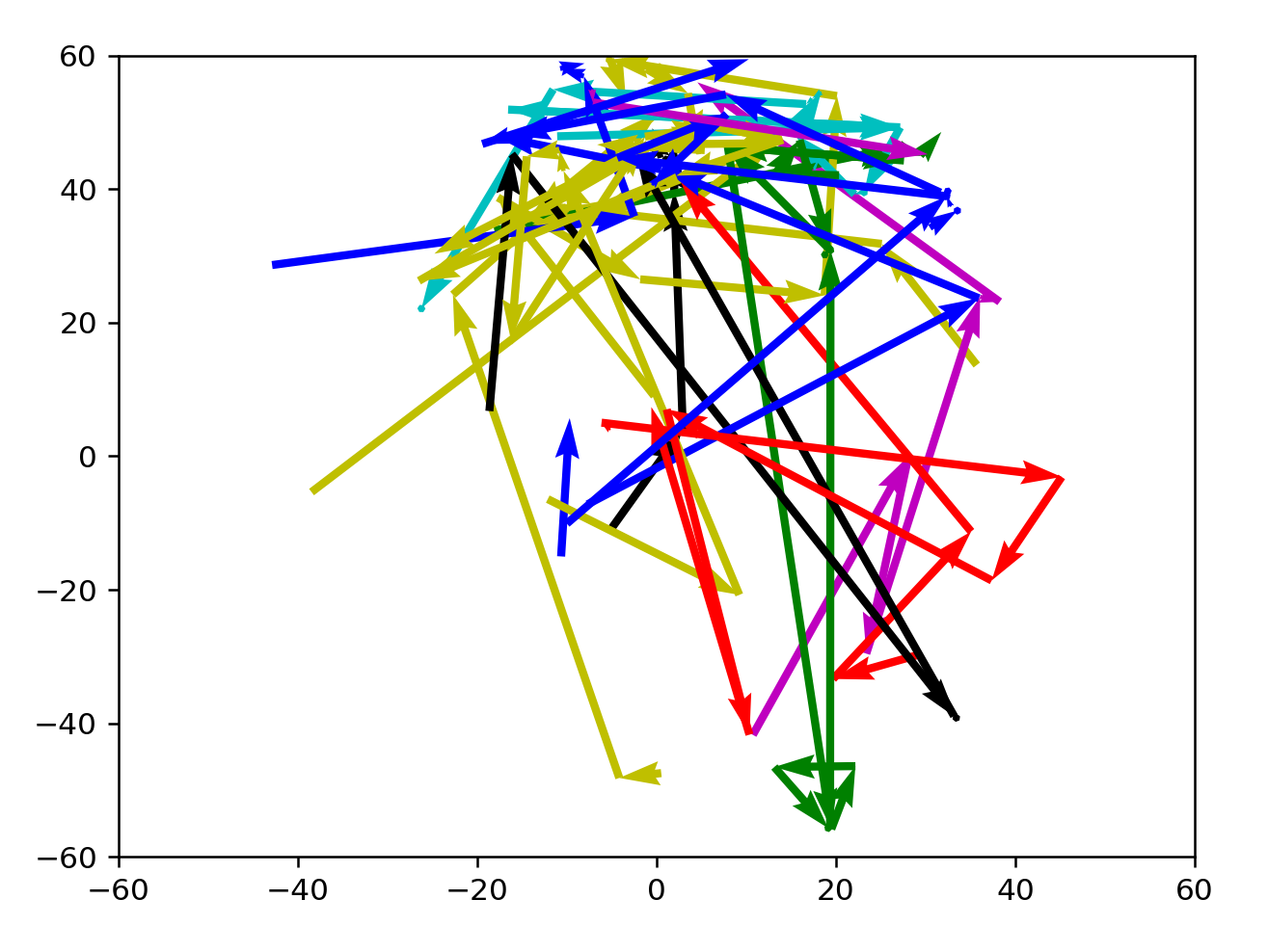
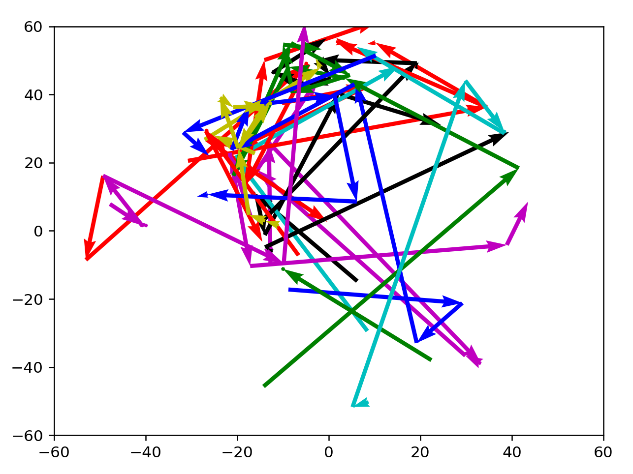
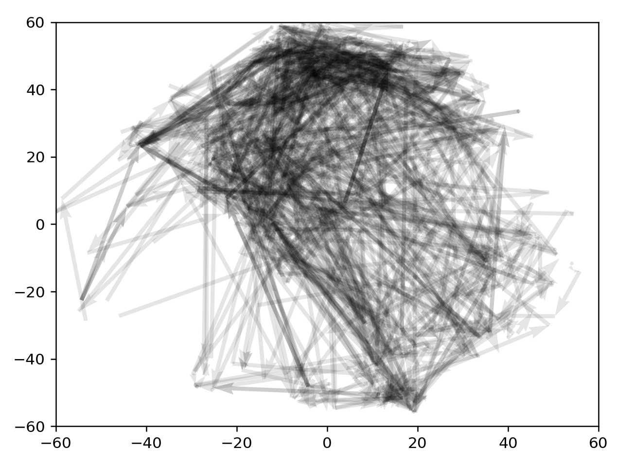
Let's try verifying that BFS solutions look good instead.
These results are better, but not inherently satisfying yet. Compared to a random selection of coordinates in wordspace, the path that these jumps are taking looks really good. However, it's not golf-like enough and it isn't clear how to make the lines straighter.
Taking a break
Here are a few things that could have happened. My visualization code is not working is a possibility. My BFS search not working is another possibility. I could be wrong in general, and dimensionality reduction can't capture semantic direction very well. This would mean a physical analogue wouldn't work with TSNE at least. However, there is definitely an idea of wordspace that can be captured intuitively, just not right now with the current tools I'm trying. This has to be an inherent quality to the word model.
I used the wrong model
I don't know why this didn't occur to me earlier but this is not actually the correct model I should be using if I want to run historical data on it. Chances are the GloVe model has significantly different directions than Word2Vec, so what I just did was actually testing the more tenuous hypothesis that not only is there a geographic analogue to semantic space, there's also a universal geographic analogue between different models. That question can wait. I will do some BFS runs on the Word2Vec model in a bit and put those graphs up here.
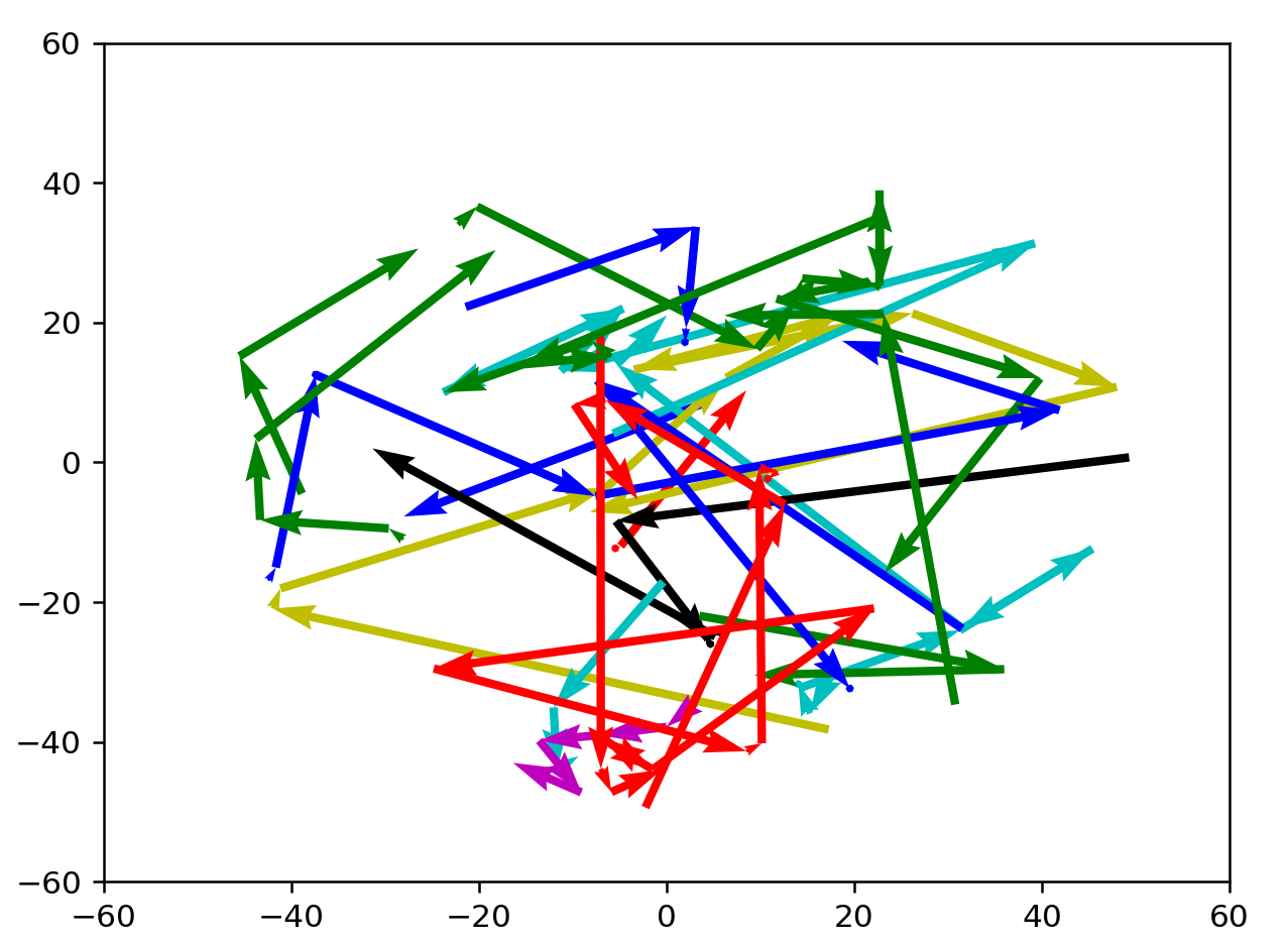
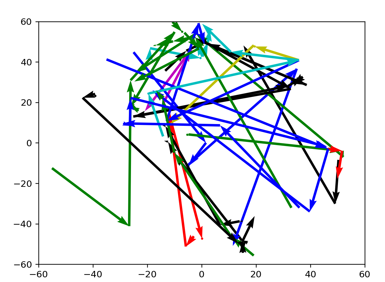
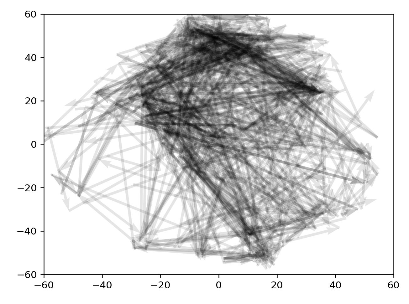
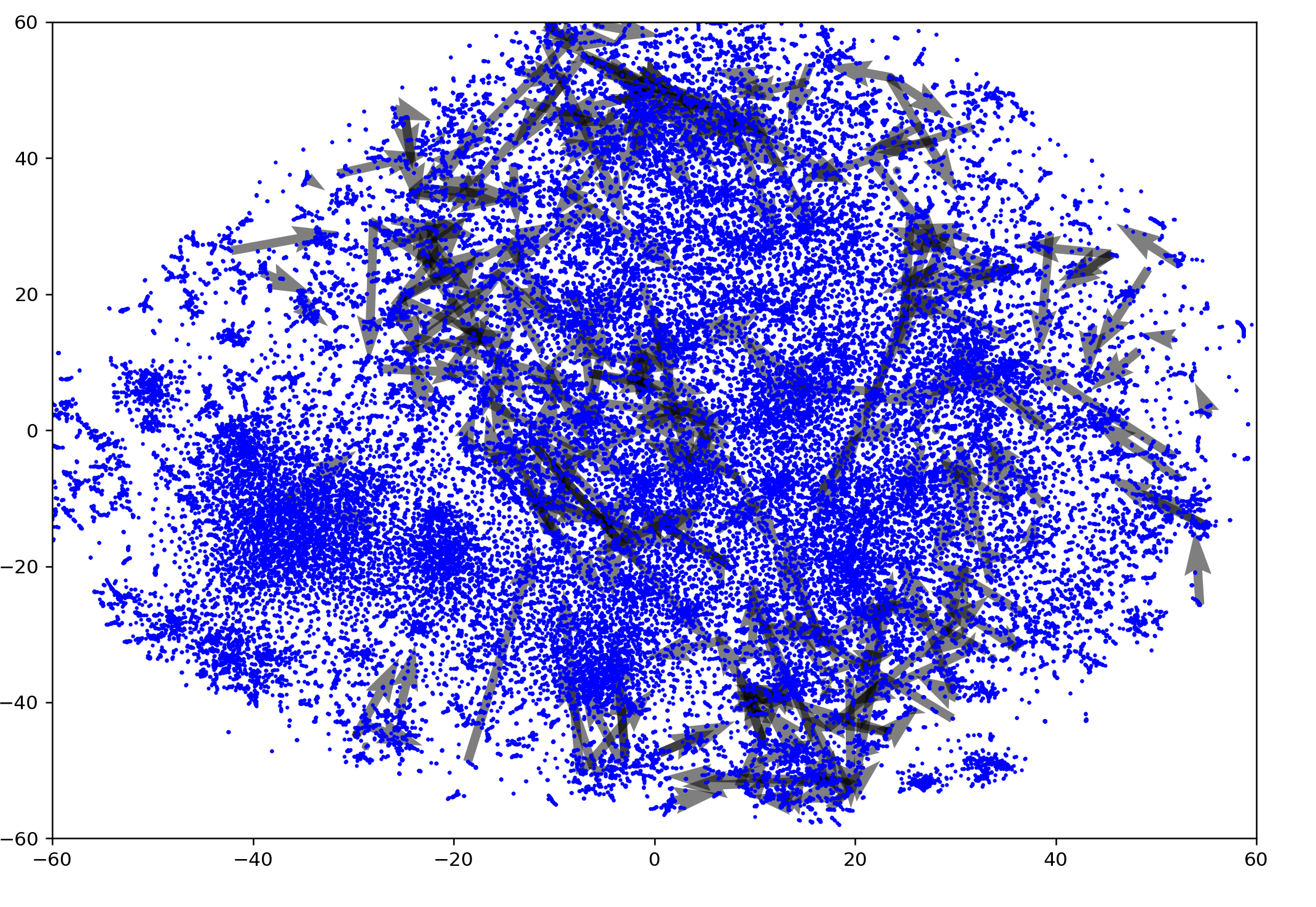
golf maps for correct model
These are not BFS runs, but just taking the data from different prompts, out of a set of about 8000 total.
3+ from 2200:2220
3+ from 3200:3220
3+ from 4200:4220
3+ from 5200:2220
3+ from 6200:3220
3+ from 7200:4220
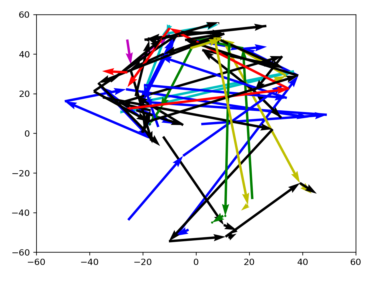
As expected, directions are well-defined here. Many arrows are clustered towards the north, which might indicate a preference for active, formal language. There seems to be a current sweeping NE, or from warm informal to cold informal words, with a few word vectors outside that enter the current before reaching a destination. Actually, this current could simply be nouns from the language.
transparency for 3+ from 1100:1400
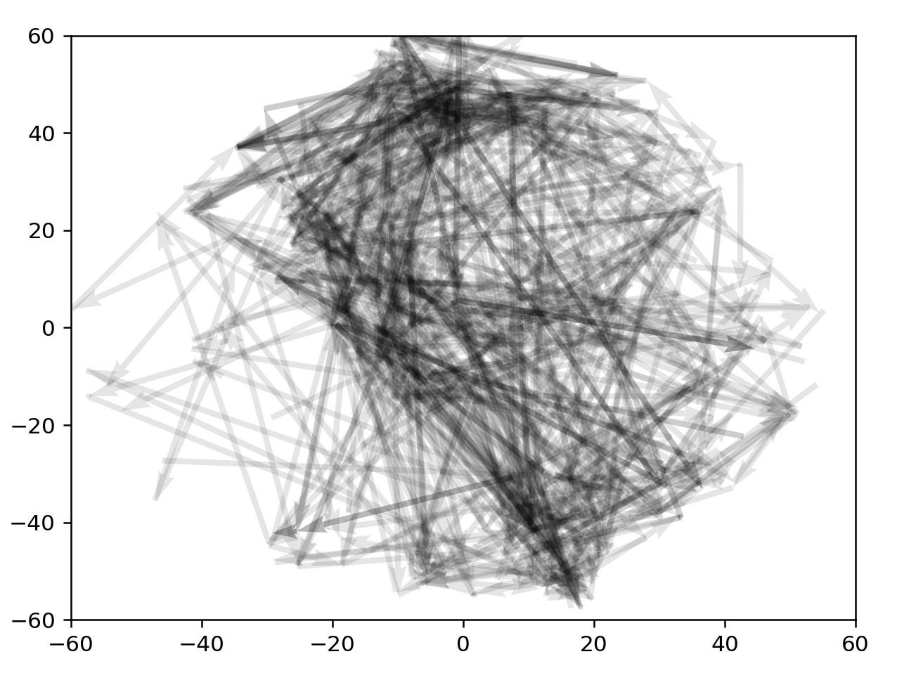
2100:2400
3100:3400
4100:4400
Annotating glove
Let's do this the slow, sure way. We can annotate by part of speech to begin with. Here are the coordinates we have to work with to begin with:
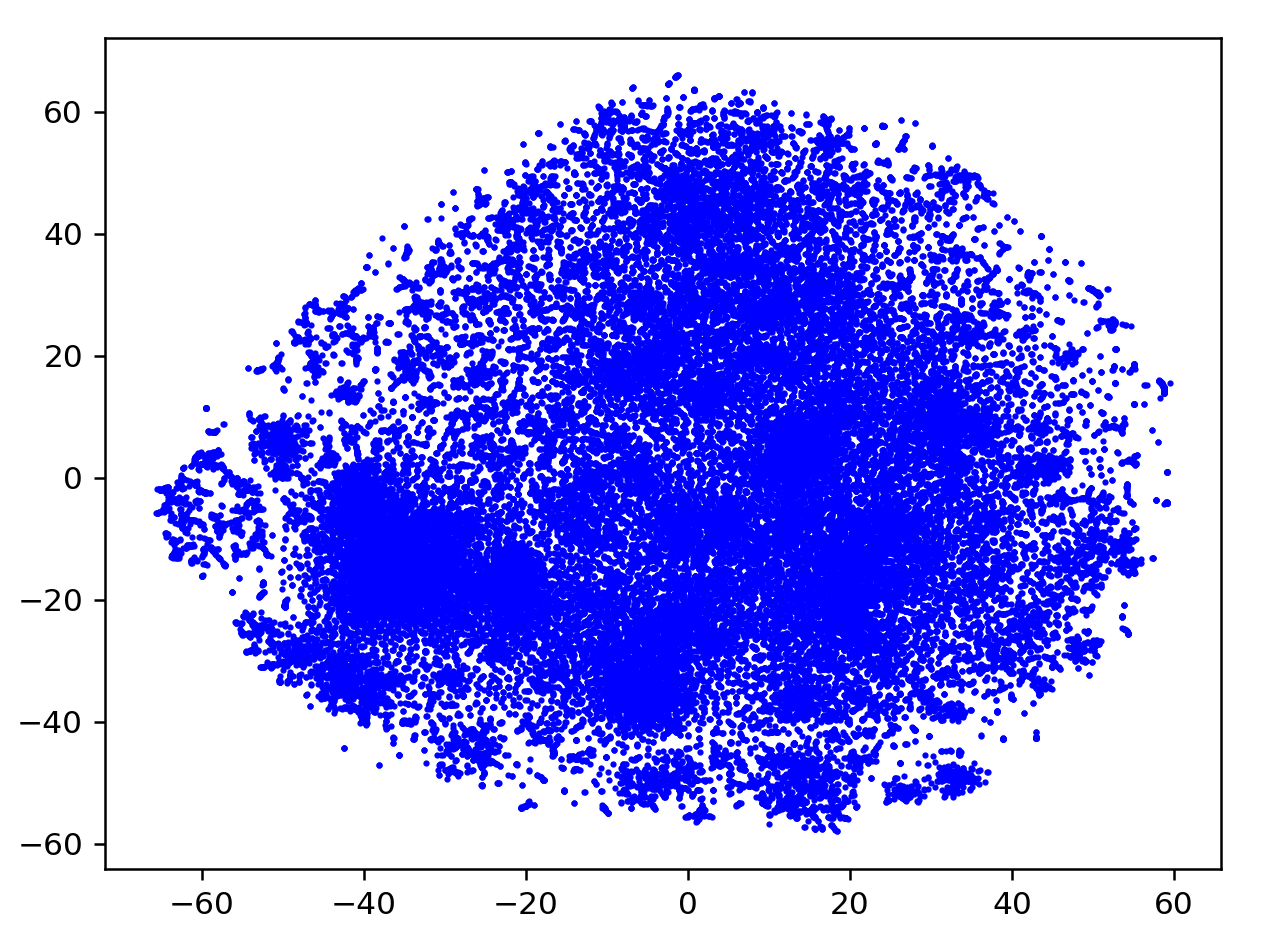
This visualization makes me feel sick
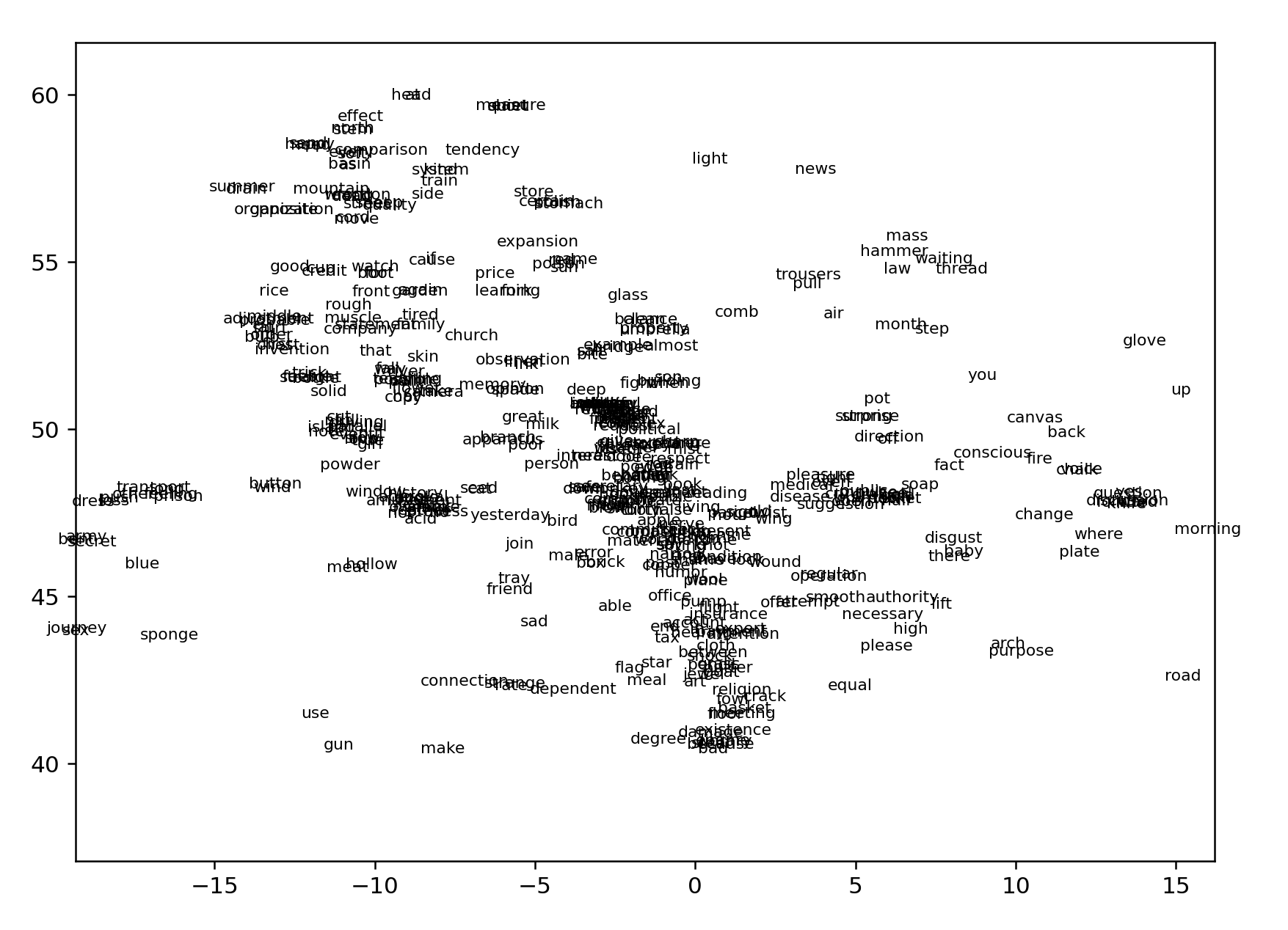
Promisingly, the current does not correlate with the largest clusters. Now, as with the Esperanto cluster set but without the aggluginative shortcut, we can write an NLTK script to classify different words and then graph them in different colors. Actually wait. We can just graph the words and take a look first. For all words that appear more than one out of ten thousand (zipf > 5):
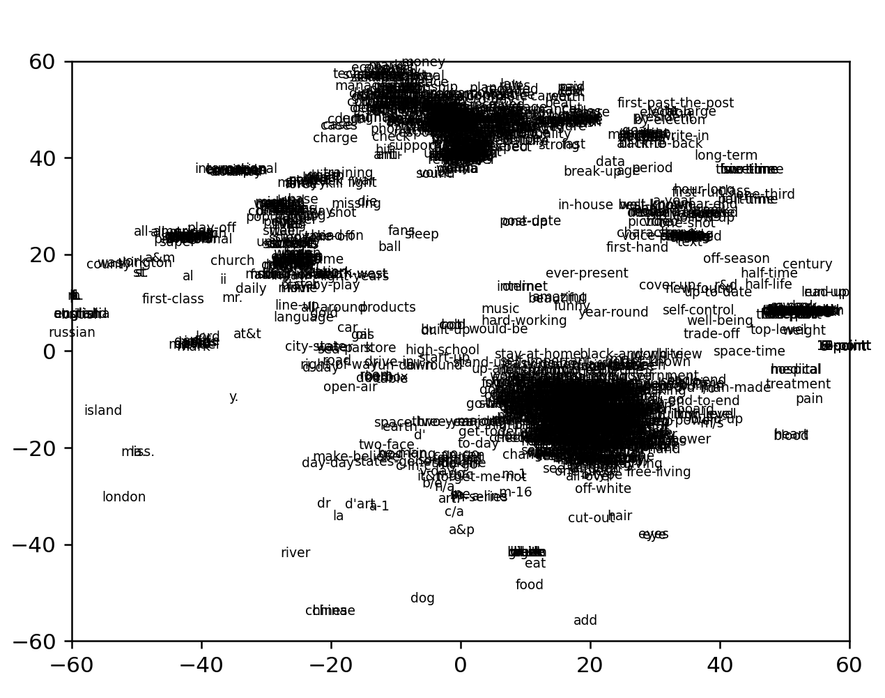
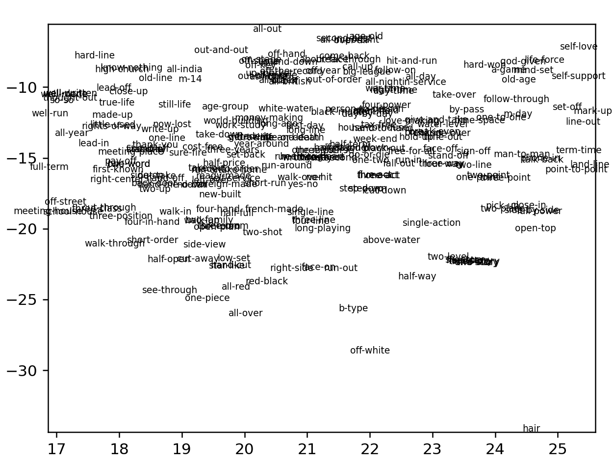
Zooming in on the bottom right chunk reveals it to be mostly hyphenated words:
Top are newspaper nouns, top-left are more general nouns
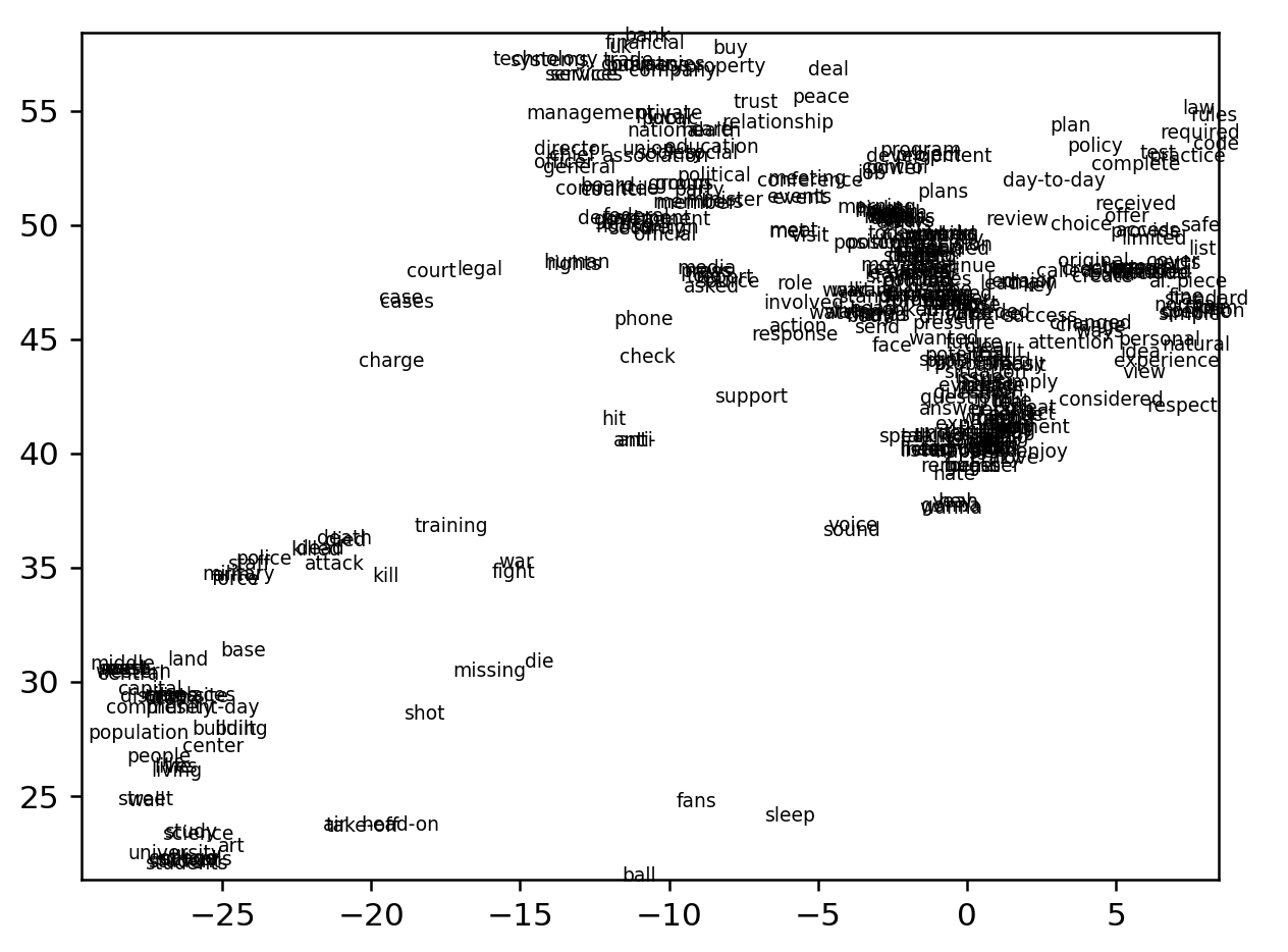
Bottom section are all food and nature terms
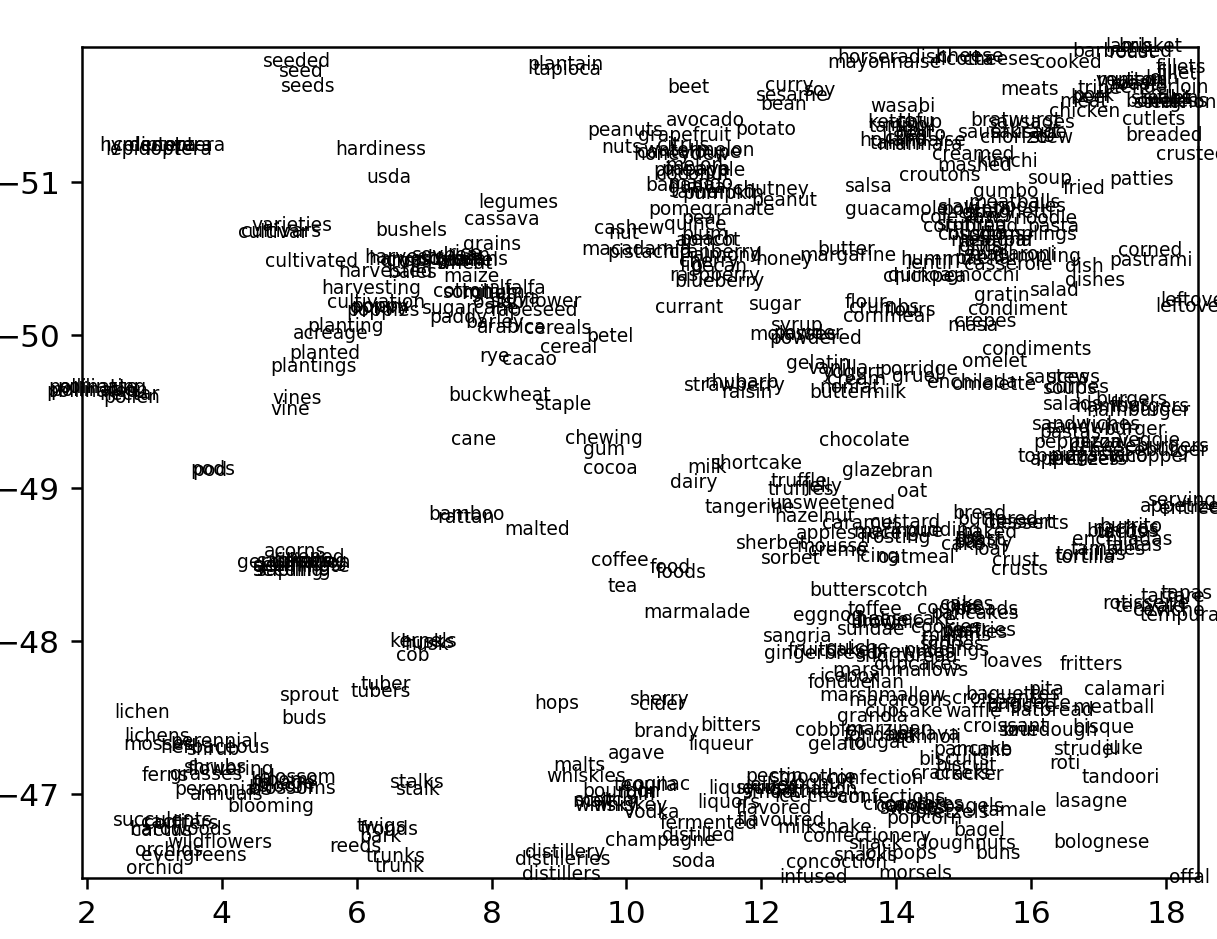
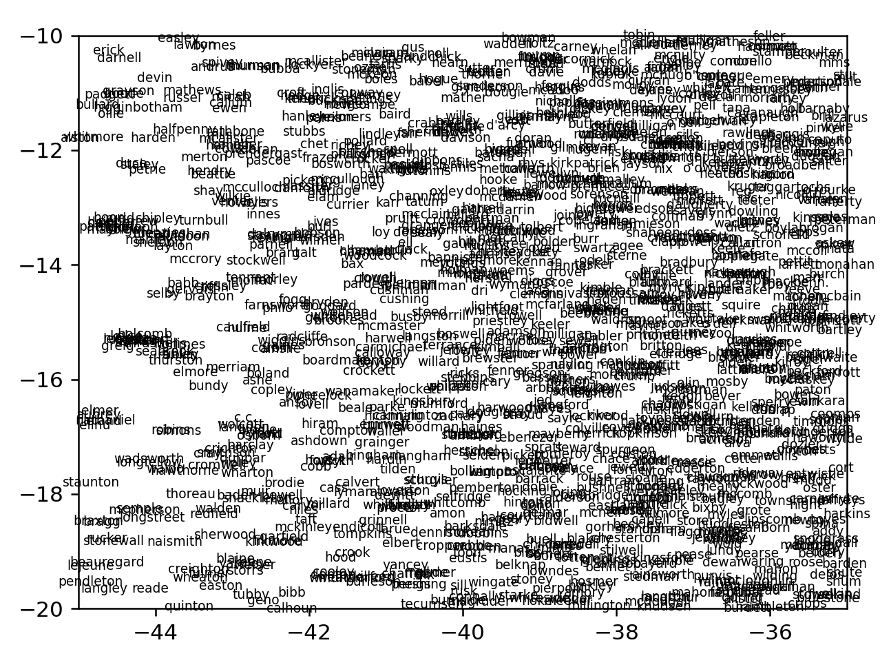
Bottom-left are names
Visualizing Ogden's Simple English Set
I tired myself out now. There's so much more work to be done, including finding models in other languages and actually creating a way to interact with these models geographically through arrow keys. Let's try something simpler that might reveal more information.
Last night I was using a simplified set of 850 words from Ogden's Basic English and thinking about whether there are applications in language learning here that haven't been explored. The advantage of this set is that there are no names and the words have been carefully curated to form a core structure for the English language. So let's put up a graph of those words. I'm guessing they will be a cresent in the top NE corner.
Ogden (n=839) with ogden positions
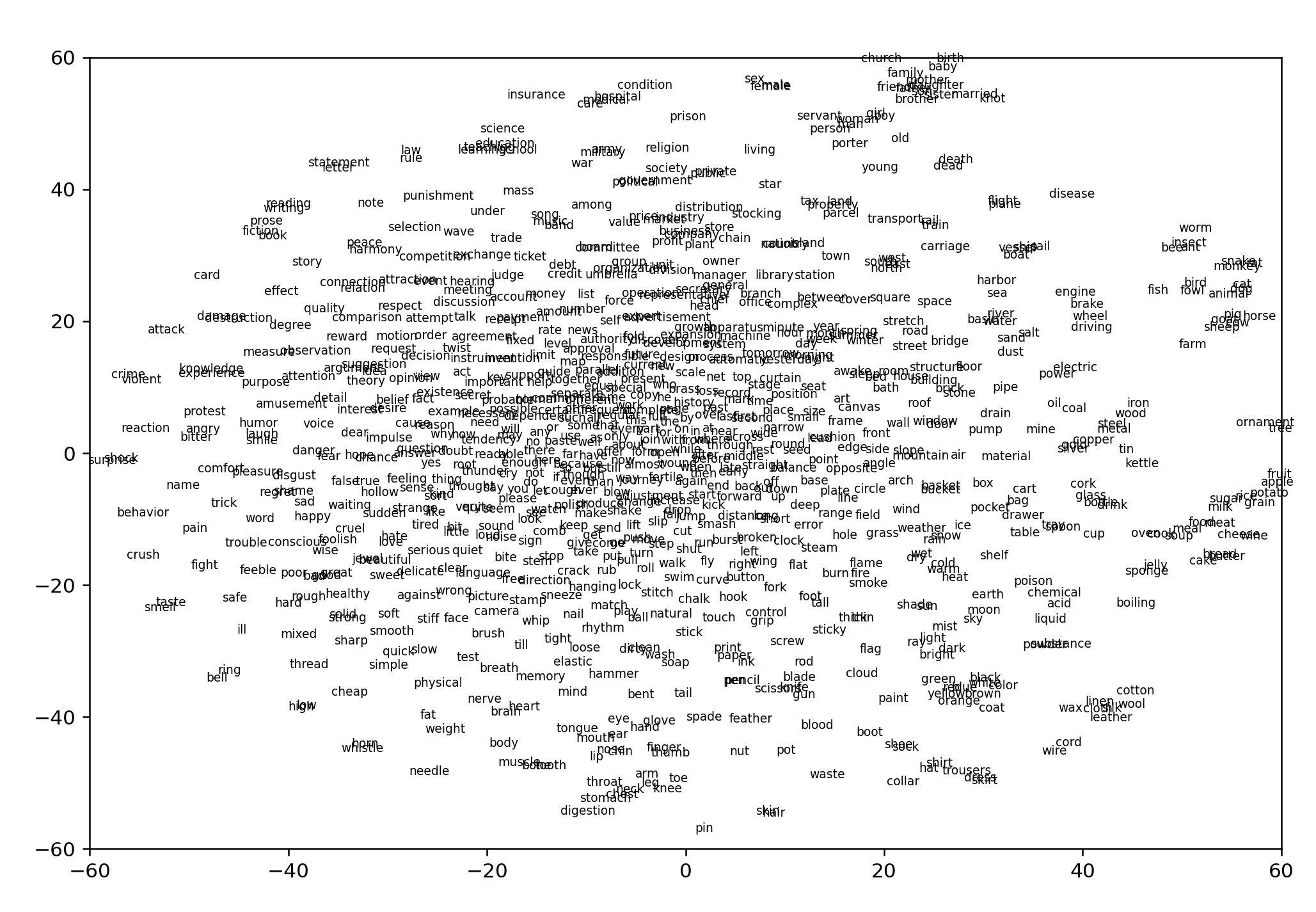
Ogden with glove positions
Okay wait a second. This is fascinating. Aside from forming the expected crescent, many of these common, curated, words delineate the outer edges of the cloud. More over, along the east and the south edges, these words are evenly spaced. This has such a great potential to serve as the semantic scale for the english language!
Looking only at the words at the very ends of the cloud:
EAST: the, well, carriage, time, kettle, space
SOUTH: color, tin, range
    cluster: till, (servant, animal), toe, ice, heart,
WEST: healthy, stiff
SOUTHWEST CLUSTER : blade, chain, but
WEST CLUSTER: serious, part, cruel, right, new
	supercluster: (under, foolish, house, punishment, snake, roll, lead)
	supercluster: (W/E) (breath, hanging, plant, detail, song, school, smell, leather, only, answer, advertisment, (rule, stage, laugh, sticky, special))
NORTH: summer, (send,happy,need), effect, (head, at), (quiet, short, measure), man, light, news
distinctive ridge S/N here, on the south end of ridge: (damage, steel, bad, because, english, library, existence, meeting, basket)
NORTHEAST CLUSTER: year, roof, bag, moon, far, after, wine, south, judge, unit, table, any, early
Zooming into S/N ridge at top:
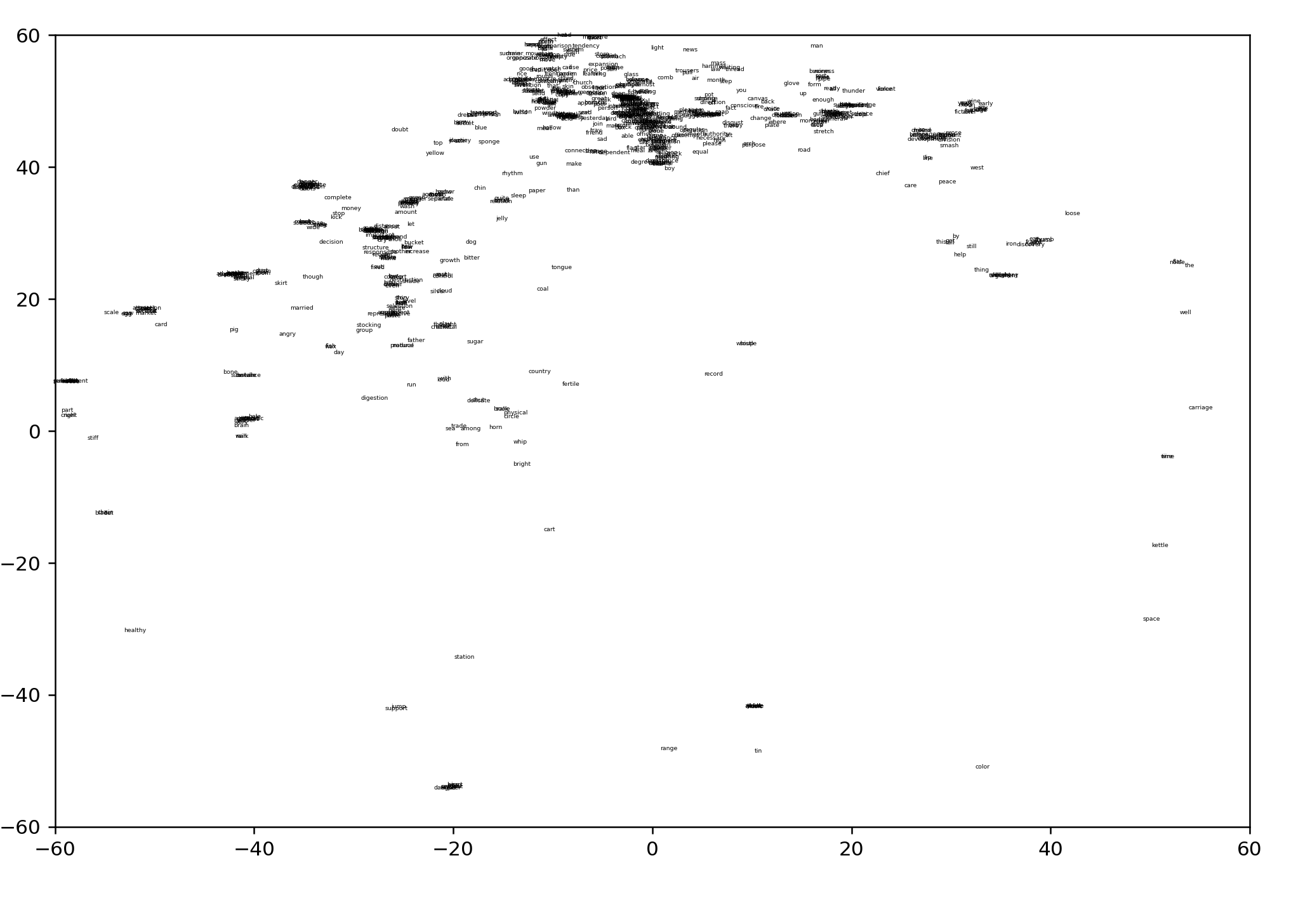
Now what happens if we take these same ogden words and visualize them against word2vec?
visualizing ogden against word2vec
We have the following words to visualize:
the,well,carriage,time,kettle,space,color,tin,range,till,servant,animal,toe,ice,heart,healthy,stiff,blade,chain,but,serious,part,cruel,right,new,under,foolish,house,punishment,snake,roll,lead,breath,hanging,plant,detail,song,school,smell,leather,only,answer,advertisment,rule,stage,laugh,sticky,special,summer,send,happy,need,effect,head,at,quiet,short,measure,man,light,news,damage,steel,bad,because,english,library,existence,meeting,basket,year,roof,bag,moon,far,after,wine,south,judge,unit,table,any,early
This is our result:
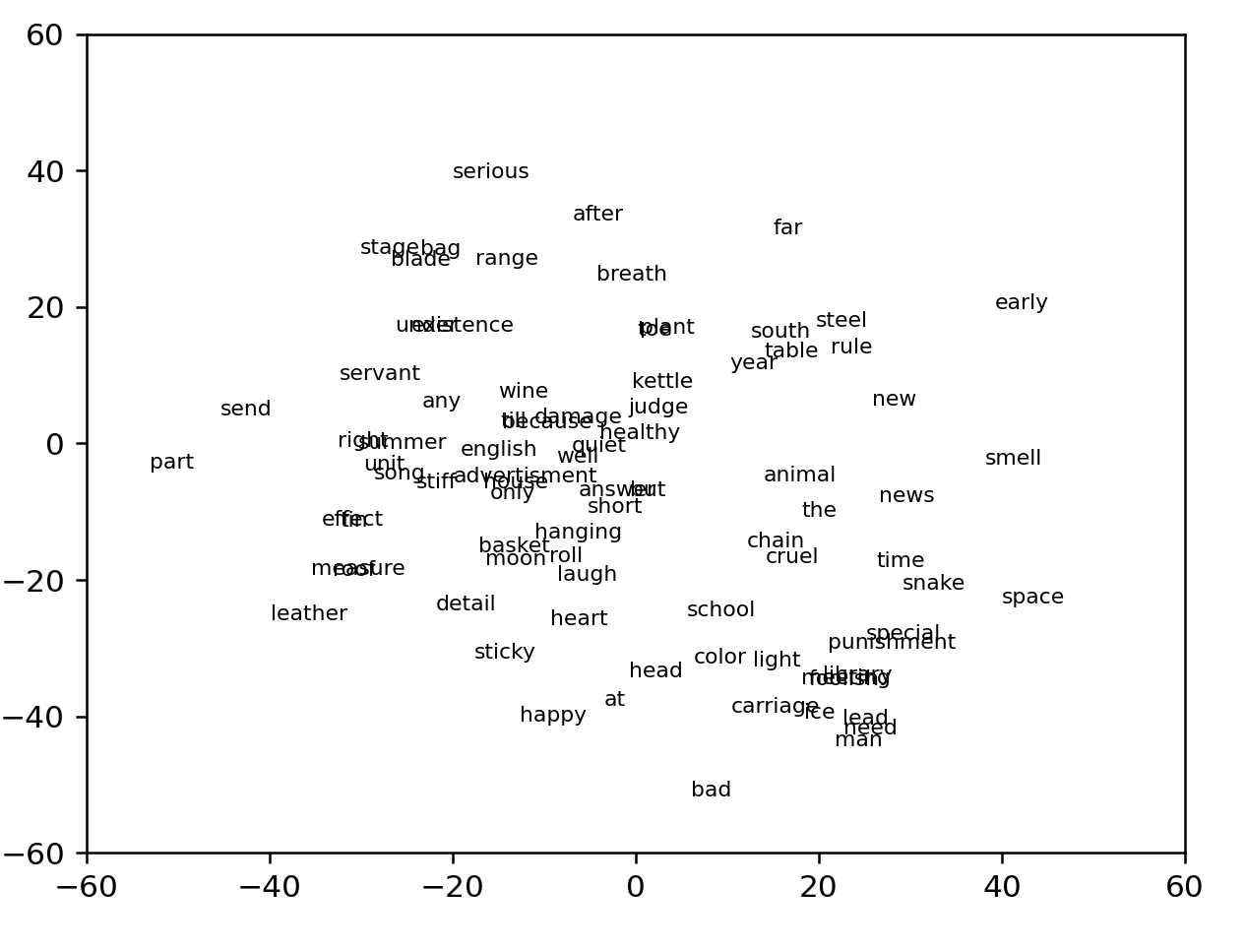
This quite obviously fails to produce the same boundaries, which is to be expected. Oh well. One immediate difficulty with viewing these words as a scale, however, is that we already know roughly what two of the largest clusters are -- names, and food -- and it's not immediately clear how such a scale would be useful in navigating these clusters.
Compass for the production model: word2vec filtered to 2.3 with 32,000 words
Following the same procedure as above we can obtain cardinal outliers for our production model:
WEST: droplet,droplets,ionic,transistors,transistor,ion,ionized
EAST: brothers,grandparent,cousins,sons,sisters,aunts,siblings
SOUTH: partition,partitioning,partitioned,holder,holders,bowled
NORTH: sorority,sororities,greeks,greek,birdies,pars,bogey,bogeys
Now we want to retrieve nearest neighbors in various directions. We can first write a nearest neighbor script:
    def distance(r1,r2):
        return ((r1[0]-r2[0])**2 + (r1[1]-r2[1])**2)**(1/2)

    def nearest_2Dneighbor(word):
        min_distance = 10
        neighbor = ""
        for index in wv.key_to_index:
            v1 = tsneFlat[wv.key_to_index[word]]
            v2 = tsneFlat[wv.key_to_index[index]]
            d = distance(v1, v2)
            if d < min_distance and index != word:
                min_distance = d
                neighbor = index
        print(f'closest to {word} is {neighbor} with distance {min_distance}')
Verifying, we can see it works:
closest to zebra is hippo with distance 0.07393014825495706We can get multiple neighbors by reading and writing to a dict:
    def nearest_2Dneighbors(word, ct):
    min_distances = {100:"dog"}
    for index in wv.key_to_index:
        v1 = tsneFlat[wv.key_to_index[word]]
        v2 = tsneFlat[wv.key_to_index[index]]
        d = distance(v1, v2)
        if d < max(min_distances) and index != word:
            min_distances[d] = index
            if len(min_distances) > ct:
                max_key = max(min_distances.keys())
                min_distances.pop(max_key, None)
    print(f'closest to {word} are {min_distances}')
    nearest_2Dneighbors("zebra",10)

    closest to zebra are {0.3994482615370888: 'elephant', 0.4810890428610893: 'silverback', 0.5629074693562021: 'gorillas', 0.11746016150593233: 'hippos', 0.1818965679307882: 'giraffe', 0.4521648164696161: 'elephants', 0.4599412267344633: 'rhinos', 0.07393014825495706: 'hippo', 0.41851106296130747: 'rhino', 0.37239726128557654: 'rhinoceros'}
Trying for a gridification of the graph
    WORD = "candle"
    coords = tsneFlat[wv.key_to_index[WORD]]
    neighbors = nearest_2Dneighbors(WORD,4)
    #X,Y, name
    coordlist = list(neighbors.values())
    Xcoords = [s.split(",")[0] for s in coordlist]
    Ycoords = [s.split(",")[1] for s in coordlist]
    names = [s.split(",")[2] for s in coordlist]

    for i in range(0, 100):
        WORD = names[random.choice(range(0,8))]
        coords = tsneFlat[wv.key_to_index[WORD]]
        neighbors = nearest_2Dneighbors(WORD,9)
        coordlist = list(neighbors.values())
        names = [s.split(",")[2] for s in coordlist]
        print(f"{WORD},", end="")
        for name in names:
            print(name, end=",")
        print("")

    combine = []
    combineX = []
    for i in range(0,len(Xcoords)):
        combine.append(float(Xcoords[i])*float(Ycoords[i]))
        combineX.append(float(Xcoords[i])*float(Ycoords[i])*float(Xcoords[i]))
    #represent words in a grid
    Xdiffs = [float(coords[0]) - float(Xcoord) for Xcoord in Xcoords]
    Ydiffs = [float(coords[1]) - float(Ycoord) for Ycoord in Ycoords]
    cw, ccw = [], []
    #check which rotation is closer
    quadrants = [0,0,0,0]
    for i in range(0, 4):
        if (Xdiffs[i] > 0 and Ydiffs[i] > 0): quadrants[i] = 1 #north
        if (Xdiffs[i] > 0 and Ydiffs[i] < 0): quadrants[i] = 2 #east
        if (Xdiffs[i] < 0 and Ydiffs[i] < 0): quadrants[i] = 3 #south
        if (Xdiffs[i] < 0 and Ydiffs[i] > 0): quadrants[i] = 4 #west

    #clockwise swing
    def swing(indice):
        return abs(np.arctan(Xdiffs[indice]/Ydiffs[indice]))

    #print(quadrants)
    while len(quadrants) != len(set(quadrants)):
        for i in range(0, 4):
            #if a quadrant has multiple
            if quadrants.count(quadrants[i]) > 1:
                #print(f"too much in quadrant {quadrants[i]}")
                #while more than one in same quadrants, move the closer one (indice wrt quadrants & diffs)
                indices = [index for index, element in enumerate(quadrants) if element == quadrants[i]]
                #given indices for a quadrant, we want to find the index with the minimum swing, and move that quadrant
                #print(f"indices are {indices}")
                swings = [swing(indice) for indice in indices]
                minSwingIndex = indices[swings.index(min(swings))]
                quadrants[minSwingIndex]+=1
                #print(f"point with indice {minSwingIndex} moved from {quadrants[minSwingIndex]} to {quadrants[minSwingIndex]+1}")
                if(quadrants[minSwingIndex]) > 4:
                    quadrants[minSwingIndex] = 1
    #print("_    "+names[quadrants.index(1)])
    #print(names[quadrants.index(4)] + f"<--{WORD}-->" + names[quadrants.index(2)])
    #print("_    "+names[quadrants.index(3)])
From four quadrants it should derive four directions, but these directions don't yet form a grid.
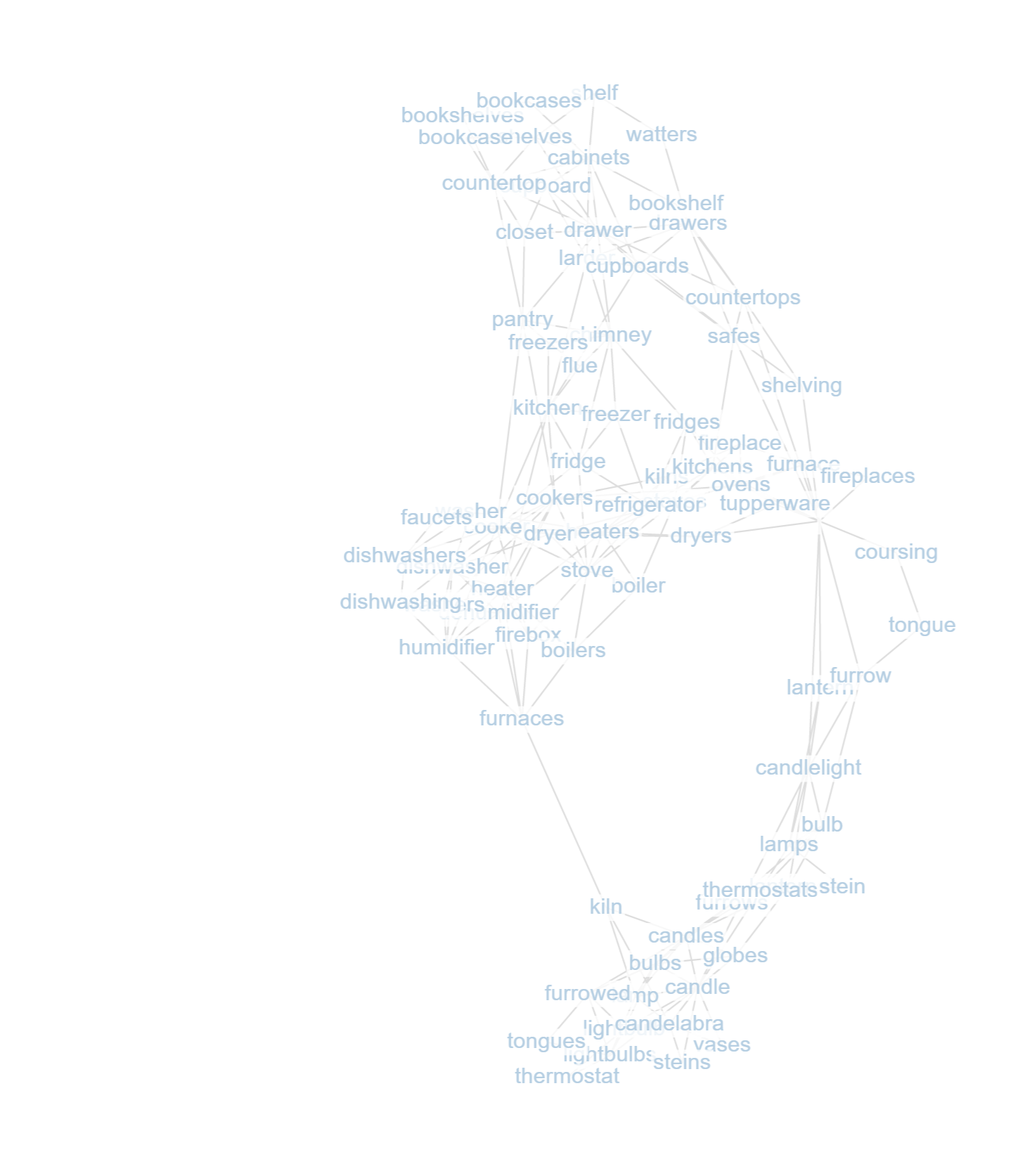
salvaging graphview for the quick visualization of close neighborhoods
Access this utility tool at /graphviz.html. Built with force-graph.js from the previous view used in golf
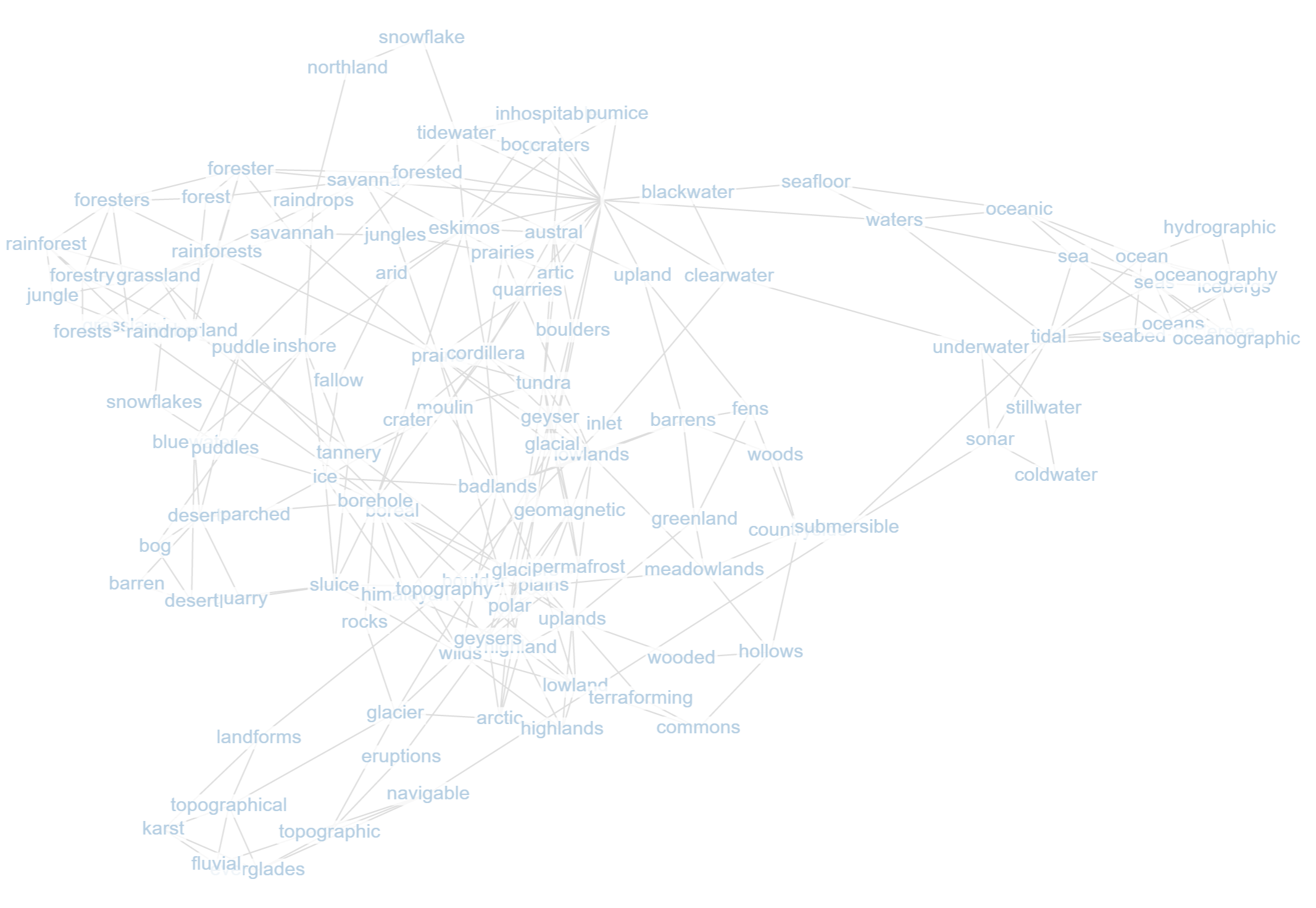
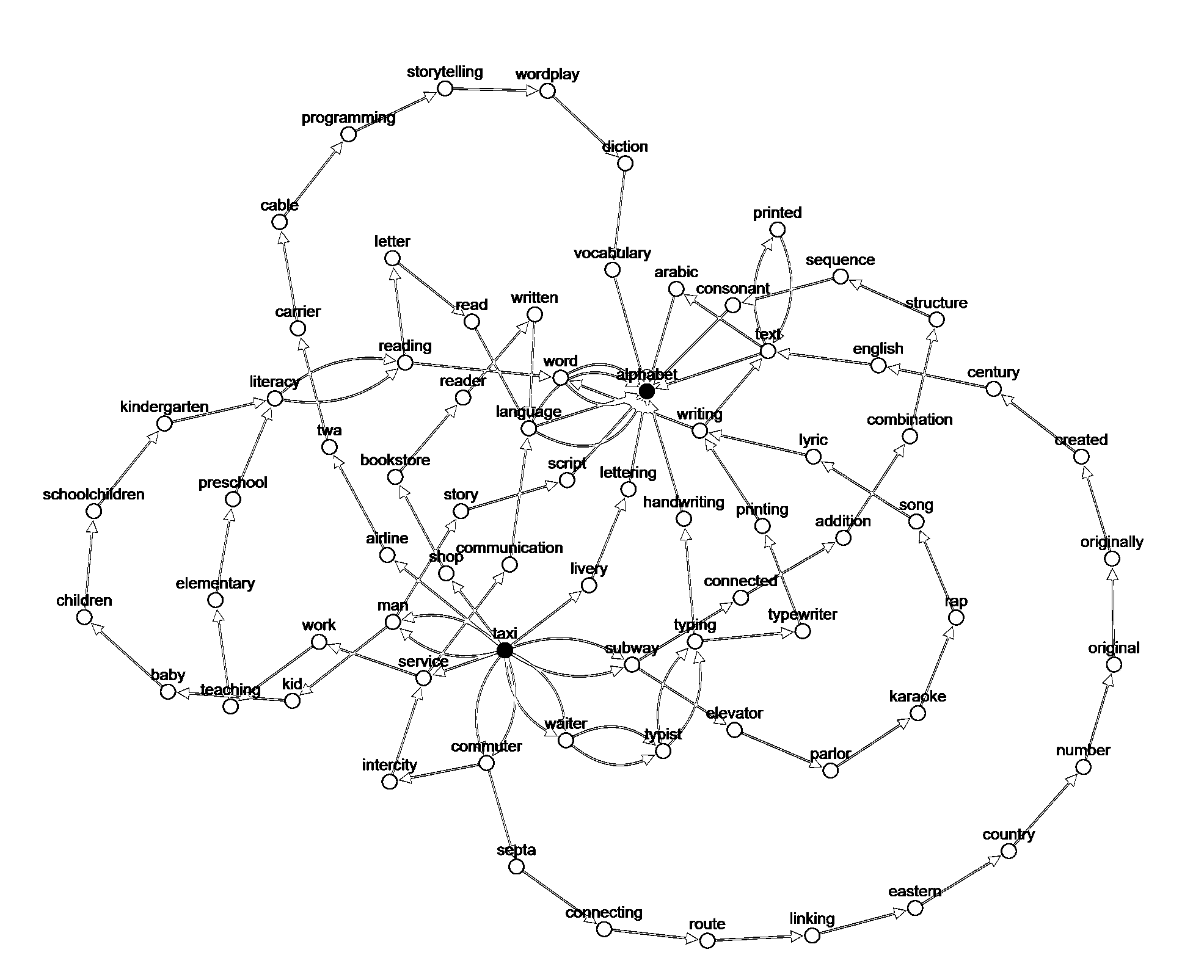
For 100 random walks with view depth 9 at "candle":
For 100 random walks with view depth 9 at "rainforest":